Introduction to Information Theory

Some of the notes I wrote when I took an information theory course. It contains basic definitions and theorems. It doesn’t get into much details and is sort of an intuitive cheat-sheet. The content aligns with the first few chapters of the book “Elements of Information Theory” by Cover and Thomas, so you can find the proofs there (it is a very well-written and easy-to-read book, I definitely recommend it!).

Entropy

Let $X$ be a discrete random variable with alphabet $\mathcal{X}$ and probability mass function $p(x)$.

The entropy $H(X)$ of a discrete random variable $X$ is defined by $H(X) = -\mathbb{E}_{X\sim p(x)}\left[\log p(X)\right] = - \sum_{x\in\mathcal{X}}p(x)\log p(x).$

Intuitively, the entropy $H(X)$ is a measure of how informative the observation of an instantiation of $X$ is. Alternatively, we can think of it as how uncertain we are about the value of $X$.
If $X$ is not random at all, we already know what an instantiation is going to be; therefore, the entropy is zero. On the other hand, the more uniformly distributed $p(x)$ is, the more uncertain we are about the value of an instantiation of $X$.
When calculating the entropy, we don’t consider the values of $x\in \mathcal{X}$ for which $p(x) = 0$. So, conventionally, $0\log 0 = 0\log\infty = 0$ and $p\log\infty = \infty$ in the calculations.

Joint and Conditional Entropy

The joint entropy $H(X, Y)$ of a pair of random variables is just the entropy of their joint distribution:

\[H(X, Y) = -\mathbb{E}_{X\sim p(x), Y\sim p(y)}\left[\log p(X, Y)\right] = \sum_{x\in\mathcal{X}, y\in\mathcal{Y}}p(x, y)\log p(x, y).\]

The conditional entropy of $Y$ given $X$ is defined as the expected entropy of $Y$ given the value of $X$:

\[H(Y\mid X) = -\mathbb{E}_{X\sim p(x), Y\sim p(y)}\left[\log p(Y\mid X)\right] \\ = -\sum_{x\in\mathcal{X}, y\in \mathcal{Y}}p(x, y)\log p(y\mid X) \\ = \sum_{x\in \mathcal{X}}p(x)H(Y\mid X=x).\]

In general, $H(Y\mid X) \neq H(X\mid Y)$. For example, consider $X \sim \mathrm{Uniform} (\{1, \cdots, 100 \})$ and $Y=X \;\mathrm{mod}\; 10$.

Because of the natural definition of entropy, many of the theorems about probability distributions translate naturally for entropy. For instance, we have the chain rule:

\[H(X, Y) = H(X) + H(Y\mid X)\]

KL-divergence and Mutual Information

The Kullback-Leibler divergence or relative entropy between two probability mass functions $p(x)$ and $q(x)$ is defined as

\[D(p\|q) = \mathbb{E}_{X\sim p(X)}\left[\log\frac{p(X)}{q(X)}\right] = \sum_{x\in \mathcal{X}} p(x)\log\frac{p(x)}{q(x)}.\]

In calculations, let $0\log {(\mathrm{whatever})} = 0$ and $p\log\frac{p}{0} = \infty$ for $p>0$.
You can think of KL-divergence as some sort of distance between $p$ and $q$. However, it is not a metric, as it is not symmetric and does not satisfy the triangle inequality.
Another way of thinking about it is as a measure of how similar samples of $p$ are to those of $q$.
If there is a symbol $x \in \mathcal{X}$ that may be seen when we sample from $p$, but will never appear when sampling from $q$ (i.e., $p(x)>0 = q(x)$), then the distance $D(p|q)$ is $\infty$. This is because there is a chance that, when sampling from $p$, we observe $x$, and immediately recognize that we are not sampling from $q$. Note however, that $D(q|p)$ may not be $\infty$, as not observing $x$ can not assure us that we are sampling form $p$.

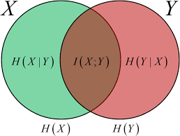
The mutual information $I(X; Y)$ between two random variables is the KL-divergence between their joint distribution, $p(x, y)$ and the product of their marginals, $p(x)p(y)$:

\[I(X; Y) = D(p(x, y)\|p(x)p(y)) = \sum_{x\in\mathcal{X}, y\in \mathcal{Y}} p(x, y)\log\frac{p(x, y)}{p(x)p(y)}.\]

Mutual information is symmetric, i.e., $I(X;Y) = I(Y;X).$
You can think of mutual information as the amount of shared information between two random variables. If $X$ and $Y$ are independent, their mutual information is zero. Otherwise, their mutual information is strictly positive.
If $Y = f(X) $ for any one-to-one mapping $f$, then $X$ and $Y$ contain the same information; hence, their mutual information is equal to (each of) their entropies.
In particular, the amount of shared information between $X$ and itself, is precisely the entropy of $X$:
\[I(X; X) = H(X)\]
The mutual information can also be thought of as the reduction in the uncertainty of one variable, due to the knowledge of the other, i.e.,
\[I(X; Y) = H(Y) - H(Y\mid X) = H(X) - H(X\mid Y).\]
We can also write the mutual information as the sum of information in each variable, minus the total information contained (jointly) in $X$ and $Y$:
\[I(X; Y) = H(X) + H(Y) - H(X, Y)\]

Conditional Divergence and Mutual Information

We can define conditional KL-divergence and conditional mutual information the same way we did for entropy.

The conditional mutual information between $X$ and $Y$ given $Z$ is the reduction in the uncertainty of $X$ due to the knowledge of $Y$, given that $Z$ is known:

\[I(X;Y\mid Z) = H(X\mid Z) - H(X\mid Y, Z) = \mathbb{E}_{X, Y, Z \sim p(x, y, z)} \left[\log\frac{p(X, Y\mid Z)}{p(X\mid Z)p(Y\mid Z)}\right]\]

The conditional KL-divergence between the conditional distributions $p(y\mid x)$ and $q(y\mid x)$ is defined to be

\[D(p(y\mid x)\|q(y\mid x)) = \mathbb{E}_{X, Y\sim p(x, y)}\left[\log\frac{p(Y\mid X)}{q(Y\mid X)}\right].\]

(Notice how the expectation is taken with regards to the joint distribution $p(x, y)$)

We also have chain rule for mutual information:

\[I(X_1,\cdots,X_n; Y) = \sum_{i=1}^{n}I(X_i;Y\mid X_1,\cdots, X_{i-1}),\]

and for the KL-divergence: $D(p(x_1, \cdots, x_n)\|q(x_1, \cdots, x_n)) = \sum_{i=1}^{n} D(p(x_i\mid x_1,\cdots, x_{i-1})\|q(x_i\mid x_1, \cdots,x_{i-1}))$ Remark: To prove any of the chain rules, just

write the quantity in question (be it entropy, divergence, or mutual information) as the expected value of a function of the joint distributions,
decompose the joint distributions inside the expectation by conditioning on variables one at a time,
logarithm of products is equal to sum of logarithms,
use linearity of expectation.

Inequalities and Bounds

There are two main inequalities that are used in to provide bounds in the context of entropies: Jensen and log-sum inequalities. Before introducing them, some definitions:

A function $f: (a, b) \to \mathbb{R}$ is convex if for every $x_1, x_2 \in (a, b)$ and $\lambda \in [0, 1]$,

\[f(\lambda x_1 +(1-\lambda) x_2) \leqslant \lambda f(x_1) + (1-\lambda)f(x_2).\]

If $f$ is twice differentiable, this is equivalent to $f''(x)\geqslant 0$ for all $x\in (a, b)$.

Intuitively, $f$ is convex if it lies below the line segment connecting any two points on its graph.

A function $f$ is concave if $-f$ is convex. This means that the inequality in the definition of convexity changes its direction, the second derivative is non-positive, and $f$ lies above the line segment connecting any two points on its graph.

Jensen’s Inequality: If $f$ is a convex function and $X$ is a random variable, $ \mathbb E [f(X)] \geqslant f(\mathbb E [X]).$ We particularly use this when $f$ is the logarithm function. If $f$ is concave, the direction of inequality changes.

Log-Sum Inequality: For non-negative numbers $a_1, a_2, \cdots, a_n$ and $b_1, b_2, \cdots, b_n$,

\[\sum_{i=1}^{n} {a_i\log\frac{a_i}{b_i}} \geqslant (\sum_{i=1}^n a_i) \log\frac{\sum_{i=1}^n a_i}{\sum_{i=1}^n b_i}\]

with equality if and only if $\frac{a_i}{b_i} = \mathrm{constant}$.

This inequality follows from the application of Jensen to the convex function $f(t) = t\log t$.

Notice how the left hand side is similar to the definition of KL-divergence!

Now, let’s see some consequences of the application of these inequalities:

KL-divergence is non-negative: $D(p|q)\geqslant 0$ with equality only when $p=q$.
Mutual information and conditional mutual information are both non-negative: $I(X; Y\mid Z)\geqslant 0$ with equality only when $X$ and $Y$ are conditionally independent given $Z$.
(Uniform distribution gives maximum entropy) $H(X) \leqslant \log \mid \mathcal{X}\mid $ where $\mathcal{X}$ is the support of $X$ and equality if and only if $X$ is the uniform distribution over $\mathcal{X}$.
(Conditioning reduces entropy) Intuitively, having information about $Y$ can only decrease the uncertainty in $X$: $H(X\mid Y) \leqslant H(X)$.
(Independence bound on entropy) The joint entropy of $n$ variables can not be any larger than the sum of their individual entropies:
\[H(X_1, \cdots, X_n) \leqslant \sum_{i=1}^n H(X_i)\]
with equality if and only if $X_i$’s are independent.
(Convexity of KL-divergence) $D(p|q)$ is convex in the pair $(p, q)$; that is, for any two pairs of distributions $(p_1, q_1)$ and $(p_2, q_2)$ and any $\lambda \in [0, 1]$,
\[D(\lambda p_1 +(1-\lambda)p_2 \| \lambda q_1 + (1-\lambda)q_2) \leqslant \lambda D(p_1\|q_1) + (1-\lambda) D(p_2\|q_2).\]
(Concavity of entropy) $H(p)$ is a concave function of $p$. Thus, the entropy of mixture of distributions is as large as the mixture of their entropies. This result follows easily from the convexity of KL-divergence, because:
Let $u$ be the uniform distribution over $\mathcal{X}$. For any distribution $p$ over $\mathcal{X}$,
\[H(p) = H(u) - D(p\|u) = \log {\mid \mathcal{X}\mid } - D(p\|u)\]

Data-Processing Inequality

Let $X\rightarrow Y \rightarrow Z$ be a Markov chain, that is, $Z$ is independent of $X$ given $Y$: $p(x, y, z) = p(x)p(y\mid x)p(z\mid y)$. Then,

\[I(X;Y) \geqslant I(X;Z).\]

The data processing inequality shows that no clever manipulation of the data can improve the inference that can be made with that data.
In particular, for any function $g$, $X \rightarrow Y \rightarrow g(Y)$ is a Markov chain, thus
\[I(X; Y) \geqslant I(X, g(Y))\]
which yields the previous claim about data manipulation.

Fano’s Inequality

Suppose we know a random variable $Y$ and we want to guess the value of a correlated random variable $X$. Intuitively, knowing $Y$ should allow us to better guess the value of $X$. Fano’s inequality relates the probability of error in guessing $X$ to the conditional entropy $H(X\mid Y)$.

Suppose we use $\hat{X} = g(Y)$ to estimate $X$ after observing $Y$ ($g$ is a possibly random function). One can see that $X \rightarrow Y \rightarrow \hat X$ forms a Markov chain. We would like to bound the probability of error in estimating $X$ using $\hat X$, defined as

\[P_e = Pr[\hat X \neq X]\]

(Fano’s inequality) For any estimator $\hat X$ such that $X\rightarrow Y \rightarrow \hat X$ forms a Markov chain, we have

\[H(P_e) + P_e \log {\mid \mathcal{X}\mid } \geqslant H(X\mid \hat X) \geqslant H(X\mid Y).\]

This can be weakened to

\[1 + P_e \log {\mid \mathcal X\mid } \geqslant H(X\mid Y)\]

\[P_e \geqslant \frac {H(X\mid Y) - 1}{\log {\mid \mathcal{X}\mid }}.\]

So, the larger $H(X\mid Y)$ is, the more likely it is for our estimator to make an error.

Notice that $I(X; Y) = H(X) - H(X\mid Y)$. So, if we fix the entropy of $X$, large mutual information between $X$ and $Y$ indicate that we can better estimate $X$ given $Y$.