<?xml version="1.0" encoding="utf-8"?><feed xmlns="http://www.w3.org/2005/Atom" xml:lang="en"><generator uri="https://jekyllrb.com/" version="4.4.1">Jekyll</generator><link href="https://conflictednerd.github.io/feed.xml" rel="self" type="application/atom+xml" /><link href="https://conflictednerd.github.io/" rel="alternate" type="text/html" hreflang="en" /><updated>2026-11-18T06:37:35+00:00</updated><id>https://conflictednerd.github.io/feed.xml</id><title type="html">Saeed Hedayatian</title><subtitle>PhD candidate in Computer Science at University of Southern California</subtitle><entry><title type="html">Variational Inference</title><link href="https://conflictednerd.github.io/blog/2023/Variational-Inference/" rel="alternate" type="text/html" title="Variational Inference" /><published>2023-03-07T01:19:15+00:00</published><updated>2023-03-07T01:19:15+00:00</updated><id>https://conflictednerd.github.io/blog/2023/Variational-Inference</id><content type="html" xml:base="https://conflictednerd.github.io/blog/2023/Variational-Inference/"><![CDATA[<h2 id="preliminaries">Preliminaries</h2>
<p>It is usually the case that we have a dataset $\mathcal{D} = \{x_1, \cdots, x_N \}$ and a parametrized family of distributions $p_\theta (x)$. We would like to find the parameters that best describe the data. This is typically done using maximum likelihood estimation (MLE). In this method, the optimal parameters are those that maximize the log likelihood of the data. Mathematically speaking,</p>

\[\hat{\theta}_\mathrm{MLE} = \arg\max_\theta \frac{1}{N}\sum_{i=1}^{N}\log p_{\theta}(x_i).\]

<p>If $p_\theta(x)$ is a simple distribution like a Gaussian for which the likelihood can be written in an analytic form, there are no problems and we can find the MLE using an optimization technique of choice. But in many cases, the data cannot be approximated with a simple distribution like a Gaussian. For instance, consider the distribution of images in dataset like MNIST. We often say that they reside on a <strong>data manifold</strong> that can be very complicated. No simple distribution can capture the complex nature of such data.</p>

<p><strong>Latent variable models</strong> provide one way of modelling complex data distributions. In a latent variable model we assume that there are a set of hidden variables $\mathbf{z}$ that influence the data generation process. For the MNIST dataset, the digit or the style of handwriting could be considered as latent variables. In the simplest case, we could consider the following latent variable model:</p>

\[p(x) = \int p(x\mid z)p(z)\mathrm{d}z\]

<p>But more complicated/structured models can also be considered (They are usually shown as graphical models).</p>

<p><strong>An Aside:</strong> Inferring latent variables from the a data sample (i.e., computing the posterior $p(z\mid x)$) can also be very useful. In a deep learning setting, they could provide a compact and useful representation of data. For example, in <strong>self-supervised learning</strong> it is common to learn to infer a latent representation from a large unlabeled dataset, and then train a very simple linear classifier on top of it to predict a desired label, using very few labeled samples.</p>

<p>In a latent variable model, the MLE will take the following form:</p>

\[\hat{\theta}_\mathrm{MLE} = \arg\max_\theta \frac{1}{N}\sum_{i=1}^{N}\log \int p_{\theta}(x_i\mid z)p_\theta(z)\mathrm{d}z.\]

<p>Analytically computing the above integral is in most cases very difficult or even impossible (There are some exceptions; for instance, see Gaussian mixture models). This is where variational inference comes to rescue. It circumvents the intractability issue allows us to compute the MLE of parameters.</p>

<p>Before we dive deep into the details of VI, it is useful to clearly sort out our assumptions. So in the next sections, we will see which distributions we assume have a simple tractable form and which ones are interactable/hard.</p>

<h3 id="the-knowns">The Knowns</h3>
<h4 id="pz">$p(z)$</h4>
<p>This distribution, known as the <em>prior over the latent variables</em>, is usually assumed to be a simple distribution such as $\mathcal{N}(\mathbf{0}, \mathbf{I})$. We don’t even parametrize it (no optimizing it!) and assume that it is a fixed distribution known a priori.</p>
<h4 id="p_thetaxmid-z">$p_\theta(x\mid z)$</h4>
<p>This is usually known as the <em>likelihood</em>, and it is the probability that our model generates a data point $x$, <strong>given the latent $z$</strong>. We typically assume that this distribution belongs to a simple (parametrized) family of distributions, such as the Gaussians. To give an example, we may choose to represent them as $\mathcal{N}(\mu_\theta(z), \sigma_\theta(z))$.</p>
<h4 id="p_thetax-z">$p_\theta(x, z)$</h4>
<p>The <em>joint distribution</em> can be obtained using the Bayes rule by simply multiplying the densities of the prior and the likelihood, which are both known, tractable distributions. So we can say</p>

\[p_\theta (x, z) = p_\theta(x\mid z)p(z).\]

<p>Note that we usually use a model (e.g., a probabilistic graphical model) of this joint distribution that tells us about the relation between the latent $z$ and the observed variable $x$.</p>
<h3 id="the-unknowns">The Unknowns</h3>
<h4 id="p_thetax">$p_\theta(x)$</h4>
<p>Also known as the <em>marginal</em> or the <em>evidence</em>, this is the probability that our model has generated a data point $x$. It is called so because it can be obtained from marginalizing the joint distribution:</p>

\[p_\theta (x) = \int p(x, z)\mathrm{d}z = \int p_\theta(x\mid z)p(z)\mathrm{d}z.\]

<p>Notice that although the joint distribution is known, integrating it with respect to $z$ is interactable in all but very few cases. So effectively, the marginal distribution is not available to us.</p>
<h4 id="p_thetazmid-x">$p_\theta(z\mid x)$</h4>
<p>The probability of the latent given a data point is called the posterior distribution over the latent variables (or simply the <em>posterior</em>). We can think of it as our belief about the latent given an observation $x$. Using the Bayes rule we can write it as</p>

\[p_\theta(z\mid x) = \frac{p_\theta(x, z)}{p_\theta(x)}.\]

<p>Although the nominator is known, due to the intractability of the marginal in the denominator, we can’t compute the posterior either.</p>
<h3 id="the-goal">The Goal</h3>
<p>In VI, we want to approximate the marginal and the posterior. Having tractable approximates is very useful. For instance, we could use them to find good parameters for our model by approximating $\hat{\theta}_\mathrm{MLE}$.</p>
<h2 id="evidence-lower-bound">Evidence Lower Bound</h2>
<h3 id="overview">Overview</h3>
<p>Consider the maximum likelihood estimation of parameters $\theta$ for modelling a dataset $\mathcal{D} = \{ x_1, \cdots, x_N \}$ of samples using a latent variable model $p_\theta(x)$. But, as we mentioned earlier, the marginal distribution is interactable, so we can’t even directly compute the likelihoods $\log p_\theta(x_i)$ of the samples in our dataset given a particular set of parameters. To circumvent this issue we will try to approximate the posterior $p_\theta(z\mid x_i)$ with a simple (tractable) distribution $q_i(z)$ which can be, for instance, $\mathcal{N}(\mu_i, \sigma_i)$. We will then use $q_i$’s to derive a tractable lower bound (ELBO) on $\log p_\theta(x_i)$, which is what we actually want. Finally, instead of maximizing $\log p_\theta(x_i)$s, we will maximize these tractable lower bounds. If the bounds are sufficiently tight, then pushing up the lower bounds will also push up the actual likelihoods. Furthermore, we will see that as $q_i$ approximates the posterior $p_\theta(z\mid x_i)$ better (in the sense of KL-divergence), the ELBO bound will get tighter; to the extent that if $q_i = p_\theta(z\mid x_i)$, then ELBO will be exact.</p>

<p>There is one more trick that we will use. Instead of considering a different $q_i$ to approximate the posterior given each sample in the dataset, we will use a parametrized family $q_\phi(z\mid x)$ to represent all of them at once. We can think of it as using a neural net with parameters $\phi$ that will output the mean and standard deviation of the approximate posterior given each sample, so that $q_i = q_\phi(x_i) = \mathcal{N}(\mu_\phi(x_i), \sigma_\phi(x_i))$. This trick, known as <strong>amortized variational inference</strong>, will help us optimize  $q_i$s (to tighten our bound) in a much more efficient manner.</p>
<h3 id="derivation">Derivation</h3>
<h4 id="approach-1-bounding-the-log-likelihood">Approach 1: Bounding the Log-Likelihood</h4>
<p>As we said in the overview, we ultimately want to give a lower bound for $\log p(x_i)$ (the subscript of $\theta$ is dropped for convenience). So. let’s start from this quantity and try to introduce $q_i(z)$ along the way.</p>

\[\begin{align*}
\log p(x_i) &amp;= \log \int_z p(x_i\mid z)p(z) \\
&amp;= \log \int_z p(x_i\mid z)p(z)\frac{q_i(z)}{q_i(z)} \\
&amp;= \log \mathbb{E}_{z\sim q_i} \left[\frac{p(x_i\mid z)p(z)}{q_i(z)}\right] &amp;&amp;\text{Definition of expected value} \\
&amp;\geqslant \mathbb{E}_{z\sim q_i}\left[\log\frac{p(x_i\mid z)p(z)}{q_i(z)}\right] &amp;&amp;\text{Jensen inequality} \\
&amp;= \mathbb{E}_{z\sim q_i}\left[\log p(x_i\mid z) +\log p(z) \right] - \mathbb{E}_{z\sim q_i}[q_i(z)] \\
&amp;= \mathbb{E}_{z\sim q_i}\left[\log p(x_i\mid z) +\log p(z) \right] + \mathcal{H}(q_i)
\end{align*}\]

<p>($\mathcal{H}(\cdot)$ denotes the entropy)</p>

<p>Take a look at the last expression in the derivation above. Every term used there is tractable: $p(x_i\mid z)$ is the likelihood given the latent, $p(z)$ is the prior over the latent, and $q_i$ is any distribution of our choice. This expression is called the <strong>evidence lower bound (ELBO)</strong> and is usually denoted as $\mathcal{L}_i(p, q_i)$.</p>

<blockquote>
  <p>Note that we can get a Monte Carlo estimate of the expected value terms by sampling different $z$’s from $q_i$ and averaging the respective $\log p(x_i\mid z)p(z)$ values.</p>
</blockquote>

<p>So, we defined the ELBO as</p>

\[\mathcal{L}_i(p, q_i) = \mathbb{E}_{z\sim q_i}\left[\log p(x_i\mid z) +\log p(z) \right] + \mathcal{H}(q_i),\]

<p>and established that</p>

\[\log p(x_i) \geqslant \mathcal{L}_i(p, q_i).\]

<p>This result, in itself, lets us use any distribution $q_i(z)$ to get a tractable lower bound for $\log p(x_i)$. But how tight is this bound? and how should we choose $q_i$? The basic intuition is that $q_i(z)$ should approximate the posterior $p(z\mid x_i)$, in the sense of KL-divergence. So, the ideal $q_i$ would minimize $D_\mathrm{KL} (q_i(z)\| p(z\mid x_i))$. This intuition will be made rigorous in the next section, where we take a different approach to derive ELBO.</p>

<h4 id="approach-2-kl-minimization">Approach 2: KL minimization</h4>
<p>Following the intuition given above, let’s examine $D_\mathrm{KL} (q_i(z)\|p(z\mid x_i))$ more closely.</p>

\[\begin{align*}
D_\mathrm{KL} (q_i(z)\|p(z\mid x_i)) &amp;= \mathbb{E}_{z\sim q_i}\left[\log\frac{q_i(z)}{p(z\mid x_i)}\right] \\
&amp;= \mathbb{E}_{z\sim q_i} \left[\log\frac{q_i(z)p(x_i)}{p(x_i, z)}\right] &amp;&amp;\text{Bayes' Rule} \\
&amp;= \mathbb{E}_{z\sim q_i}\left[\log\frac{q_i(z)p(x_i)}{p(x_i\mid z)p(z)}\right] &amp;&amp;\text{Bayes' Rule} \\
&amp;= \mathbb{E}_{z\sim q_i}[\underbrace{-\log p(x_i\mid z) - \log p(z) + \log q_i(z)}_{-\mathcal{L_i(p, q_i)}} + \underbrace{\log p(x_i)}_{\text{constant}}] \\
&amp;= -\mathcal{L}_i(p, q_i) + \log p(x_i) \\
&amp;\implies \log p(x_i) = \mathcal{L}_i(p, q_i) + D_\mathrm{KL}(q_i(z) \| p(z\mid x_i)).
\end{align*}\]

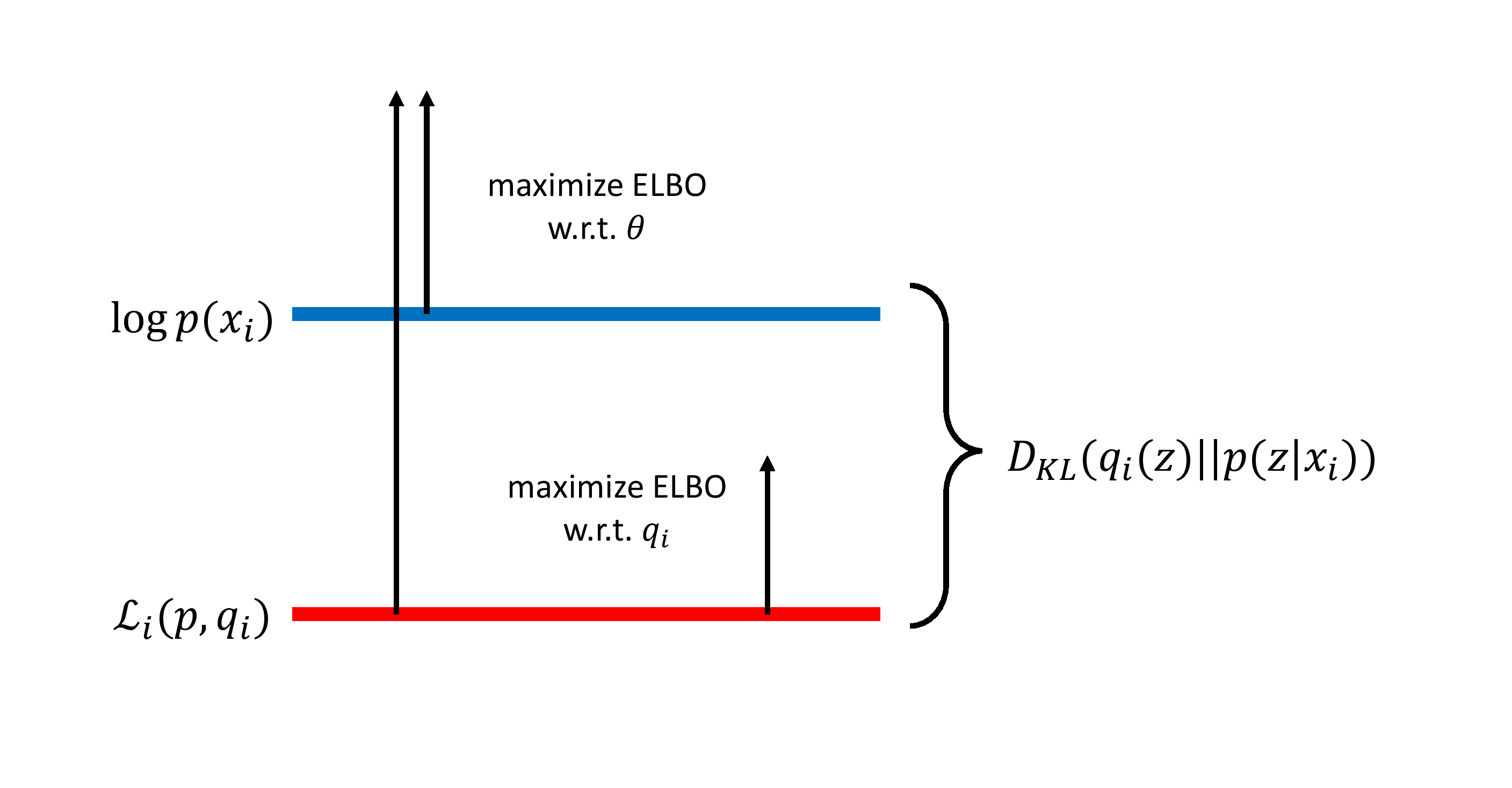
<p>Therefore $D_\mathrm{KL} (q_i(z) \| p(z \mid x_i))$ is actually the approximation error when we use $\mathcal{L}_i(p, q_i)$ instead of $\log p(x_i)$.</p>

<p>This suggests a natural optimization scheme to push up the value of $p_\theta (x_i)$: we can alternate between maximizing</p>

\[\mathcal{L}_{i} (p_\theta, q_i)\]

<p>w.r.t. $q_i$ to tighten the bound (which is equivalent to minimizing the KL), and maximizing</p>

\[\mathcal{L}_{i} (p_\theta, q_i)\]

<p>w.r.t. $\theta$ to push up the lower bound.</p>

<div class="text-center">
  <img src="/assets/img/blog/vi1.png" class="img-fluid" style="max-width: 70%;" />
</div>

<p>To sum it all up, take a look at the algorithm below.</p>
<ul>
  <li>for each $x_i$ (or minibatch)
    <ul>
      <li>calculate $\nabla_\theta\mathcal{L}_{i} (p, q_i)$ by
        <ul>
          <li>sample $z \sim q_i$</li>
          <li>let \(\nabla_{\theta} \mathcal{L}_{i} (p, q_{i}) \approx \nabla_{\theta} \log p_{\theta} (x_i \mid z)\)</li>
        </ul>
      </li>
      <li>let $\theta \leftarrow \theta + \alpha \nabla_\theta \mathcal{L}_i(p, q_i)$</li>
      <li>update $q_i$ to tighten the bound by
        <ul>
          <li>let $q_i \leftarrow \arg \max_{q_i} \mathcal{L}_i(p, q_i)$</li>
        </ul>
      </li>
    </ul>
  </li>
</ul>

<p>This algorithm could have been fully practical if not for the last step. We have not specified how one should update $q_i$ to maximize $\mathrm{ELBO}$ (or to minimize the KL). In the special case when $q_i \sim \mathcal{N} (\mu_{i}, \sigma_{i})$, we can analytically compute</p>

\[\nabla_{\mu_{i}} \mathcal{L}_{i} (p, q_{i})\]

<p>and</p>

\[\nabla_{\sigma_{i}} \mathcal{L}_{i} (p, q_{i})\]

<p>and use them to update parameters (here, mean and variance) of \(q_i\) using gradient ascent. But even this requires us to store one set of parameters for each $q_i$, resulting in a total of \(N \times (\mid \mu_{z} \mid  + \mid \sigma_{z} \mid )\). This means that the number of parameters grows with the size of the dataset, which is impractical. In the next section, we will maintain exactly how $q_i$’s should be updated and use amortized inference to manage the number of parameters.</p>

<h4 id="amortized-vi">Amortized VI</h4>
<p>The idea of amortized variational inference is to use a network parametrized by $\phi$ to represent the approximate posterior for all data points. This would break the dependence of the number of parameters to the size of the dataset. This network, denoted by $q_\phi(z\mid x)$ would take as input a data point $x$ and output the distribution $q_i(z)$. A common choice, used in VAEs is to have</p>

\[q_\phi(z\mid x) = \mathcal{N} (\mu_\phi(x), \sigma_\phi(x)).\]

<p>Using amortized VI would changing the last step of the algorithm presented above to $\phi \leftarrow \arg\max_\phi \mathcal{L}(p_\theta(x_i\mid z), q_\phi(z\mid x_i))$. Similar to how we updated $\theta$, we use gradient ascent to optimize $\phi$. For this, we would need to compute</p>

\[\nabla_\phi \mathcal{L}(p_\theta(x_i\mid z), q_\phi(z\mid x_i)).\]

<p>The final missing piece to complete our algorithm is to calculate this gradient. So let’s examine it more closely.</p>

\[\begin{align*}
&amp;\nabla_\phi \mathcal{L}(p_\theta(x_i\mid z), q_\phi(z\mid x_i)) \\
&amp;= \nabla_\phi \underbrace{\mathbb{E}_{z\sim q_\phi(z\mid x_i)}\left[\log p_\theta(x_i\mid z) + \log p(z)\right]}_{J(\phi)} + \nabla_\phi\underbrace{\mathcal{H}(q_\phi(z\mid x_i))}_{\text{entropy of Gaussian}}.
\end{align*}\]

<p>Notice that the second term is just the gradient of the entropy of a Gaussian distribution which has a closed analytical form (If we are using automatic differentiation tools, computing this gradient would be very easy). Therefore we focus on the first term. To compute the first term we can use <strong>policy gradient theorem</strong> which would yield</p>

\[\nabla_\phi J(\phi) = \mathbb{E}_{z\sim q_\phi(z\mid x_i)} \left[\left(\log p_\theta(x_i\mid z) + \log p(z)\right)\nabla_\phi q_\phi(z\mid x_i)\right].\]

<p>The expected value on the right hand side can be estimated by sampling from $q_\phi(z\mid x_i)$, which is easy to do as it is a normal distribution with mean $\mu_\phi(x_i)$ and standard deviation $\sigma_\phi(x_i)$. So the policy gradient theorem would give us the following estimate of the gradient</p>

\[\nabla_\phi J(\phi) \approx \frac{1}{M}\sum_{j=1}^{M} \left(\log p_\theta(x_i\mid z_j) + \log p(z_j)\right)\nabla_\phi q_\phi(z\mid x_i)\]

<p>where $z_j$’s are sampled from $q_\phi(z\mid x_i)$.</p>

<p>The policy gradient estimator is known to have a high variance. For our purposes, a better estimator can be obtained through <strong>reparameterization trick</strong>.<br />
The main intuition behind reparameterization trick is that we can view a sample $z$ from $q_\phi(z\mid x_i) = \mathcal{N}(\mu_\phi(x_i), \sigma_\phi(x_i))$ as $z = \mu_\phi(x_i) + \varepsilon \sigma_\phi(x_i)$ where $\varepsilon \sim \mathcal{N}(0, 1)$.<br />
Substituting this, we can rewrite $J(\phi)$ as</p>

\[J(\phi) = \mathbb{E}_{\varepsilon \sim \mathcal{N}(0, 1)}\left[\log p_\theta(x_i\mid \mu_\phi(x_i) + \varepsilon \sigma_\phi(x_i)) + \log p(\mu_\phi(x_i) + \varepsilon \sigma_\phi(x_i))\right].\]

<p>Because the distribution over which the expected value is defined does not depend on $\phi$ anymore, we can push the gradient operator inside it and have</p>

\[\nabla_\phi J(\phi) = \mathbb{E}_{\varepsilon \sim \mathcal{N}(0, 1)}\left[\nabla_\phi\log p_\theta(x_i\mid \mu_\phi(x_i) + \varepsilon \sigma_\phi(x_i)) + \nabla_\phi\log p(\mu_\phi(x_i) + \varepsilon \sigma_\phi(x_i))\right].\]

<p>To get a estimate of the gradient we can sample $\varepsilon_1, \cdots, \varepsilon_M \sim \mathcal{N}(0, 1)$ and write</p>

\[\nabla_\phi J(\phi) \approx \frac{1}{M}\sum_{j=1}^{M}\nabla_\phi\log p_\theta(x_i\mid \mu_\phi(x_i) + \varepsilon_j \sigma_\phi(x_i)) + \nabla_\phi\log p(\mu_\phi(x_i) + \varepsilon_j \sigma_\phi(x_i)).\]

<p>This estimator has a much lower variance and even using $M=1$ would give us a good approximation of the gradient.</p>

<blockquote>
  <p>When using the reparameterization trick in the VAEs, the ELBO is usually written in the form of the reconstruction loss and a KL term (See the next section). With this formulation, the KL term, $D_\mathrm{KL}(q_\phi(z\mid x_i)\|p(z))$, would be the divergence between two Gaussians and would again have a closed form that we could differentiate. This would simplify $J(\phi)$ as \(J(\phi) = \mathbb{E}_{\varepsilon \sim \mathcal{N}(0, 1)} [\log p_\theta(x_i\mid \mu_\phi(x_i) + \varepsilon\sigma_\phi(x_i))].\)</p>
</blockquote>

<h3 id="summary">Summary</h3>
<p>As we saw ELBO, \(\mathcal{L}_{i} (p_{\theta}, q_{\phi})\) gives a lower bound on the per-sample evidence, $p(x_{i})$.
We can write the ELBO in several different ways</p>

\[\begin{align*}
\mathcal{L} &amp;= \mathbb{E}_{z\sim q_\phi(z\mid x)} \left[\log\frac{p_\theta(x, z)}{q_\phi(z\mid x)}\right] \\
&amp;= \mathbb{E}_{z\sim q_\phi(z\mid x)} [\log p_\theta(x\mid z) + \log p(z)] + \mathcal{H}(q_\phi(z\mid x)) \\
&amp;= \log p_\theta(x) - D_\mathrm{KL}(q_\phi(z\mid x) \| p_\theta(z\mid x)) &amp;&amp; \text{Evidence minus } \mathbf{posterior} \text{ KL} \\
&amp;= \mathbb{E}_{z \sim q_\phi(z\mid x)}[\log p_\theta(x, z)] + \mathcal{H}(q_\phi(z\mid x)) &amp;&amp; \text{Avg negative energy plus entropy} \\
&amp;= \mathbb{E}_{z\sim q_\phi(z\mid x)}[\log p_\theta(x\mid z)] - D_\mathrm{KL}(q_\phi(z\mid x)\|p(z)) &amp;&amp; \text{Avg reconstruction minus } \mathbf{\text{prior}} \text{ KL}
\end{align*}\]

<p>In variational inference, maximizing ELBO with respect to $\phi$ would encourage the encoder $q_\phi$ to be like the posterior $p_\theta (z\mid x)$. Maximizing it with respect to $\theta$ could push up the evidence (used in maximizing the likelihood). To compute the gradient of ELBO with respect to $\theta$ and $\phi$, consider the average reconstruction minus prior KL formulation of it. We have</p>

\[\begin{align*}
&amp;\nabla_\theta \mathcal{L} (p_\theta, q_\phi) = \mathbb{E}_{z\sim q_\phi(z\mid x)}[\nabla_\theta\log p_\theta(x\mid z)] \\
&amp;\implies \nabla_\theta \mathcal{L} (p_\theta, q_\phi) \approx \frac{1}{M}\sum_{j=1}^{M}\nabla_\theta\log p_\theta(x\mid z_j) &amp;&amp;\text{where $z_1, \cdots, z_M \sim q_\phi(z\mid x)$}
\end{align*}\]

<p>To compute $\nabla_\phi \mathcal{L}$, taking the gradient with respect to the KL term is easy as there is a closed form expression for the KL between Gaussians. As for the gradient with respect to the first term we can either use the policy gradient theorem:</p>

\[\begin{align*}
&amp;\nabla_\phi \mathbb{E}_{z\sim q_\phi(z\mid x)}[\log p_\theta(x\mid z)] = \mathbb{E}_{z\sim q_\phi(z\mid x)}[\log p_\theta(x\mid z) \nabla_\phi \log q_\phi(z\mid x)] \\
&amp;\nabla_\phi \mathbb{E}_{z\sim q_\phi(z\mid x)}[\log p_\theta(x\mid z)] \approx \frac{1}{M} \sum_{j=1}^{M}\log p_\theta(x\mid z_j) \nabla_\phi \log q_\phi(z_j\mid x) &amp;&amp; \text{where $z_1, \cdots, z_M \sim q_\phi(z\mid x)$}
\end{align*}\]

<p>or the reparameterization trick:</p>

\[\begin{align*}
&amp;\nabla_\phi \mathbb{E}_{z\sim q_\phi(z\mid x)}[\log p_\theta(x\mid z)] = \mathbb{E}_{\varepsilon\sim \mathcal{N}(0, 1)}[\nabla_\phi\log p_\theta(x\mid \mu_\phi(x) + \varepsilon\sigma_\phi(x))] \\
&amp;\nabla_\phi \mathbb{E}_{z\sim q_\phi(z\mid x)}[\log p_\theta(x\mid z)] \approx \frac{1}{M} \sum_{j=1}^{M} \nabla_\phi\log p_\theta(x\mid \mu_\phi(x) + \varepsilon_j\sigma_\phi(x)) &amp;&amp; \text{where $\varepsilon_1, \cdots, \varepsilon_M \sim \mathcal{N}(0, 1)$}
\end{align*}\]

<h2 id="variational-autoencoder">Variational Autoencoder</h2>
<div class="text-center">
  <img src="/assets/img/blog/vae.png" class="img-fluid" style="max-width: 70%;" />
</div>

<p>For a straight forward implementation in PyTorch, check out <a href="https://towardsdatascience.com/variational-autoencoder-demystified-with-pytorch-implementation-3a06bee395ed">this tutorial</a>.
I have implemented a simple <a href="https://colab.research.google.com/drive/1YiKhOB6FsyBIZvAf1en9nbOHRvvlOwwt?usp=sharing">VAE for MNIST data using JAX and Flax</a>, which I think is a neat implementation that is close to the actual math. (though admittedly, it could have been a bit cleaner) It can serve as a baseline implementation if you want to design a more complex VAE in JAX.</p>

<p><strong>Implementation Detail:</strong> I think in implementations we usually consider the conditional to have unit variance: $p_\theta(x\mid z) = \mathcal{N}(\mu_\theta(z), I)$ so that the decoder only outputs the reconstructed version of $x$, which would effectively result in a MSE loss between $x$, $\hat x$. Also the KL does not need $\sigma_\theta$, so we don’t really lose anything by setting it to a constant. On the other hand, if we let a learnable parameter $\sigma_x$ control the variance, it will always go down as the model trains (makes sense, the smaller $\sigma_x$ is, the higher the log likelihood could get). This would mean that as training progresses, we would get larger values for the likelihood. Effectively, this is equivalent to gradually increasing the contribution of the likelihood term (vs the KL term) so that the model focuses more on reconstruction rather than being close to prior. In my experiments, this helped the VAE more accurately reconstruct the images, at the cost of a very high KL divergence. I have to examine this more, but I suspect this could actually result in less useful latents due to overfitting.</p>

<h2 id="other-resources">Other Resources</h2>
<p>Here are a few pointers to some material you can use to study variational inference.</p>

<ul>
  <li><a href="https://youtu.be/UTMpM4orS30">Lecture 18 of Berkeley’s Deep RL course</a>: Sergey Levine is a great teacher and the material he presents in this ~2 hour lecture covers most of what I discussed above with an RL flavor. I highly recommend this.</li>
  <li><a href="https://arxiv.org/abs/1906.02691">An Introduction to Variational Autoencoder</a> By Max Welling and Diederik Kingma is a great reference on VAEs. Additionally, it has a full chapter on going beyond Gaussian posteriors which is very interesting.</li>
  <li><a href="http://approximateinference.org/accepted/HoffmanJohnson2016.pdf">ELBO surgery: yet another way to carve up the variational evidence lower bound</a> This is a brief (and very nicely written!) paper that examines multiple different ways of writing the evidence lower bound.</li>
  <li><a href="https://arxiv.org/abs/1601.00670">Variational Inference: A Review for Statisticians</a> This is a more theoretical note about variational inference. David Blei is great at explaining VI and I also recommend watching some of his talks online.</li>
</ul>]]></content><author><name></name></author><category term="blog" /><category term="VI" /><category term="VAE" /><category term="Probability" /><summary type="html"><![CDATA[Variational inference and VAEs.]]></summary></entry><entry><title type="html">In Praise of Einsum</title><link href="https://conflictednerd.github.io/blog/2023/In-Praise-of-einsum/" rel="alternate" type="text/html" title="In Praise of Einsum" /><published>2023-02-19T09:10:17+00:00</published><updated>2023-02-19T09:10:17+00:00</updated><id>https://conflictednerd.github.io/blog/2023/In-Praise-of-einsum</id><content type="html" xml:base="https://conflictednerd.github.io/blog/2023/In-Praise-of-einsum/"><![CDATA[<p>This is a short note about the <code class="language-plaintext highlighter-rouge">einsum</code> functionality that is present in numpy, jax, etc. Understanding what it does is a bit tricky –naturally, because it can do the job of many other functions– but it is also very rewarding as it can help a lot with linear algebraic computations. I will use numpy’s <code class="language-plaintext highlighter-rouge">np.einsum()</code> notation, but the underlying concepts are the same regardless of slight syntactic differences in libraries.</p>

<p>Put simply, <code class="language-plaintext highlighter-rouge">einsum</code> allows you to convert simple sums over product of elements of matrices from math into code. It can also change the order of axes of a matrix (computing transposes). For instance, let’s say we want to compute the product of two matrices $A, B$ and store them in a new matrix $C$. Mathematically, we can specify $C$ as</p>

\[C_{ik} = \sum_{j} A_{ij}B_{jk}.\]

<p>In code, this could be written as <code class="language-plaintext highlighter-rouge">C = np.einsum('ij, jk -&gt; ik', A, B)</code>.
First, I will discuss exactly where we can use <code class="language-plaintext highlighter-rouge">einsum</code>. Then, I’ll explain how to use <code class="language-plaintext highlighter-rouge">einsum</code> to convert math to code and vice versa. Finally, I will show how to use <code class="language-plaintext highlighter-rouge">einsum</code> to perform some everyday linear algebraic computations.</p>

<h2 id="where">Where?</h2>
<p>Generally, speaking whenever we have a number of tensors $A^1, \ldots, A^n$ and we want to obtain a new tensor $B$ whose elements can be specified in the general form of</p>

\[B_{i_1, \ldots, i_k} = \sum_{j_1, \ldots, j_l} A^1 A^2 \ldots A^n\]

<p>then we can use <code class="language-plaintext highlighter-rouge">einsum</code> to code up the operations. This general form, which I like to call the <em>sum-of-product</em> form comes up frequently in linear algebraic computations. (Batch) matrix multiplication, matrix-vector product, vector outer-product, computing the trace, etc. are all computations that can be written in this form. In the examples section further down, a number of these applications are discussed.</p>

<h2 id="how">How?</h2>
<p>The <code class="language-plaintext highlighter-rouge">einsum</code> function takes two sets of arguments; a specification string and the tensors over which the computations are to be performed. The output of this function is a tensor containing the result. Remember the code for matrix multiplication: <code class="language-plaintext highlighter-rouge">C = np.einsum('ij, jk -&gt; ik', A, B)</code>. Here, <code class="language-plaintext highlighter-rouge">'ij, jk -&gt; ik'</code> is the specification string, <code class="language-plaintext highlighter-rouge">A, B</code> are input tensors and <code class="language-plaintext highlighter-rouge">C</code> is the output. In the explanations below, I will use this matrix multiplication code.</p>

<p>Let’s see how we can interpret the specification string. We can easily convert any <code class="language-plaintext highlighter-rouge">einsum</code> code into a sum-of-product formula by doing the following:</p>
<ol>
  <li>Write down the expression for multiplying the elements of the <strong>input tensors</strong> specified by the indices that are on the <strong>left hand side</strong> of <code class="language-plaintext highlighter-rouge">-&gt;</code> symbol in the specification string. For the matrix multiplication example, this would be \(A_{ij} B_{jk}.\)</li>
  <li>Write down the element of the output tensor specified by the indices on the <strong>right hand side</strong> of the <code class="language-plaintext highlighter-rouge">-&gt;</code> symbol. For the matrix multiplication example, this would be \(C_{ik}.\)</li>
  <li>Next we have to identify what I call <em>slack indices</em>. These are the indices that are used on the left hand side of the <code class="language-plaintext highlighter-rouge">-&gt;</code> symbol, but not on the right hand side. In other words, these are the indices that were used for the inputs in step 1, but not for the output in step 2. For the matrix multiplication example this would be the <code class="language-plaintext highlighter-rouge">j</code> index.</li>
  <li>Compute the sum of the expression in step 1 over all the slack indices to get the element of the output in step 2. For the matrix multiplication example we would write \(\underbrace{C_{ik}}_{\text{step 2}} = \sum_{\underbrace{j}_{\text{slack index}}} \underbrace{A_{ij}B_{jk}}_{\text{step 1}}.\)
And we are done! Of course, we can convert any sum-of-product expression into an <code class="language-plaintext highlighter-rouge">einops</code> code following the same logic. See the examples in the next section to get a better grip on these.
There are a couple of things that you should keep in mind:
    <ul>
      <li>In the specification string, there shouldn’t be any index on the right hand side that is not used on the left hand side. So we can’t have something like <code class="language-plaintext highlighter-rouge">ij, jk -&gt; il</code> because <code class="language-plaintext highlighter-rouge">l</code> is not used on the left hand side. This is logical if you think about it in terms of the corresponding sum-of-product equation.</li>
      <li>Dimensions of the input that correspond to the same indices in the specification string should be the same. In the matrix multiplication example, the index <code class="language-plaintext highlighter-rouge">j</code> is used in for both inputs <code class="language-plaintext highlighter-rouge">A</code> and <code class="language-plaintext highlighter-rouge">B</code>. Because of this, the corresponding dimensions (first dimension of <code class="language-plaintext highlighter-rouge">A</code> and second dimension of <code class="language-plaintext highlighter-rouge">B</code>) must have the same length, which is as if we were saying two matrices $A_{mn}, B_{kl}$ can be multiplied together, only if $n=k$.</li>
    </ul>
  </li>
</ol>

<h2 id="examples">Examples</h2>
<h3 id="matrix-vector-product">Matrix Vector Product</h3>
<p>If we have a vector $v = [v_1, \cdots, v_n]^T$ and an $m \times n$ matrix $A$, then $u = Av$ is an $m \times 1$ vector whose $i$-th element is the dot product of $v$ with the $i$-th row of $A$. Mathematically, we can represent $u$ in a sum-of-product form:</p>

\[u_i = \sum_j A_{ij} v_j.\]

<p>So the specification string is <code class="language-plaintext highlighter-rouge">'ij, j -&gt; i'</code>. Notice that here $j$ is a slack index that we sum over. The final code is <code class="language-plaintext highlighter-rouge">u = np.einsum('ij, j -&gt; i', A, v)</code>.</p>
<h3 id="inner-product">Inner Product</h3>
<p>The inner product of two $n$ dimensional vectors $u$ and $v$ is a single scalar $p$ which has a sum-of-product form:</p>

\[p = \sum_i u_i v_i.\]

<p>This means that the corresponding specification string is <code class="language-plaintext highlighter-rouge">i, i -&gt;</code>. Notice that there is no index on the right hand side of this string, which means that the output is a scalar and that $i$ is an slack index that we sum over. The final code is <code class="language-plaintext highlighter-rouge">p = np.einsum('i, i -&gt; ', u, v)</code>.</p>
<h3 id="outer-product">Outer Product</h3>
<p>If we have an $m$ dimensional vector $u$ and an $n$ dimensional vector $v$, then their outer product $A = u \otimes v$ is a rank-1, $m\times n$ matrix where the $i$-th column is $u$ multiplied by the $i$-th element of $v$. We can represent $A$ in the sum-of-product form:</p>

\[A_{ij} = u_i v_j.\]

<p>In the code, we can compute it by <code class="language-plaintext highlighter-rouge">A = np.einsum('i, j -&gt; ij', u, v)</code>. Notice that here there are no slack indices.</p>
<h3 id="row-sum-and-column-sum">Row Sum and Column Sum</h3>
<p>We can use <code class="language-plaintext highlighter-rouge">einsum</code> to compute the sum of all elements in each row. For a matrix $A$, the result would be a vector $r$ where</p>

\[r_i = \sum_j A_{ij}.\]

<p>We can turn this into a specification string and write <code class="language-plaintext highlighter-rouge">r = np.einsum('ij -&gt; i', A)</code>.
Similarly, to compute the sum of all elements in each column we can use <code class="language-plaintext highlighter-rouge">c = np.einsum('ij -&gt; j', A)</code>.
When we have multi-dimensional tensors and we want to compute their sum over an axis, <code class="language-plaintext highlighter-rouge">einsum</code> notation could help with the clarity of the code. For instance, if we write</p>
<div class="language-plaintext highlighter-rouge"><div class="highlight"><pre class="highlight"><code>Y = np.einsum('BCmn -&gt; BC', X)
</code></pre></div></div>
<p>we can immediately say that <code class="language-plaintext highlighter-rouge">A</code> has the shape <code class="language-plaintext highlighter-rouge">B x C x m x n</code> (perhaps a batch of <code class="language-plaintext highlighter-rouge">B</code> images, each with <code class="language-plaintext highlighter-rouge">C</code> channels and size <code class="language-plaintext highlighter-rouge">m x n</code>) and for each channel in each batch, we have computed the sum of all elements to arrive at a tensor that has the shape <code class="language-plaintext highlighter-rouge">B x C</code>. Contrast this with</p>
<div class="language-plaintext highlighter-rouge"><div class="highlight"><pre class="highlight"><code>Y = np.sum(X, axis=(2,3))
</code></pre></div></div>
<p>which does the same job. So <code class="language-plaintext highlighter-rouge">einsum</code> could help you track the shapes as well!</p>
<h3 id="trace">Trace</h3>
<p>The trace of a matrix $A$ is a scalar $t$ which is the sum of all elements on its main diagonal. In the sum-of-product form, this is represented by</p>

\[t = \sum_i A_{ii}.\]

<p>This can be coded as <code class="language-plaintext highlighter-rouge">t = np.einsum('ii -&gt; ', A)</code>. Notice here how the index $i$ is used twice for referencing the same input argument.</p>
<h3 id="main-diagonal">Main Diagonal</h3>
<p>Similar to the way we computed the trace, we can extract the main diagonal of a matrix as a vector. In the sum-of-product form, the main diagonal can be seen as</p>

\[d_i = A_{ii}.\]

<p>We can code this as <code class="language-plaintext highlighter-rouge">d = np.einsum('ii -&gt; i', A)</code>.</p>
<h3 id="transpose">Transpose</h3>
<p>Computing the transpose of a matrix $A$ is also very easy using <code class="language-plaintext highlighter-rouge">einsum</code>. The sum-of-product notation would simply be $B_{ji} = A_{ij}$ and the corresponding code is <code class="language-plaintext highlighter-rouge">B = np.einsum('ij -&gt; ji', A)</code>.</p>
<h3 id="batch-matrix-multiplication">Batch Matrix Multiplication</h3>
<p>Adding one (or more) batch dimension is very easy using the <code class="language-plaintext highlighter-rouge">einsum</code> notation. if <code class="language-plaintext highlighter-rouge">A</code> and <code class="language-plaintext highlighter-rouge">B</code> are batches of matrices (batch index comes first) that are to be multiplied, then we can write <code class="language-plaintext highlighter-rouge">C = np.einsum('nij, njk -&gt; nik', A, B)</code>. If we write down the corresponding sum-of-product expression, it becomes evident that the batch index just acts as a counter, not involved in the computations.</p>

\[C_{nik} = \sum_{j} A_{nij}B_{njk}\]

<p>So for the first elements in the batch $n=0$, we would have</p>

\[C_{0,ik} = \sum_{j} A_{0,ij}B_{0,jk}.\]

<p>Which means that the first element in the output batch, <code class="language-plaintext highlighter-rouge">C[0]</code>, is the matrix product of <code class="language-plaintext highlighter-rouge">A[0]</code> and <code class="language-plaintext highlighter-rouge">B[0]</code>.
We can similarly add a batch dimension to any of the other examples. There is also one nice trick when we have more than one batch dimension. We can write  <code class="language-plaintext highlighter-rouge">np.einsum('...ij, ...ji -&gt; ...ik', A, B)</code> to avoid explicitly writing all batch dimensions that proceed the last two dimensions, over which we want to perform the multiplication.</p>]]></content><author><name></name></author><category term="blog" /><category term="jax" /><category term="numpy" /><category term="machine-learning" /><summary type="html"><![CDATA[A tutorial on Einstein summation.]]></summary></entry><entry><title type="html">MAP-Elites</title><link href="https://conflictednerd.github.io/blog/2022/MAP-Elites/" rel="alternate" type="text/html" title="MAP-Elites" /><published>2022-09-29T12:47:40+00:00</published><updated>2022-09-29T12:47:40+00:00</updated><id>https://conflictednerd.github.io/blog/2022/MAP-Elites</id><content type="html" xml:base="https://conflictednerd.github.io/blog/2022/MAP-Elites/"><![CDATA[<p>MAP-Elites is an elegant algorithm for solving general optimization problems. To be more accurate, it is an <strong>illumination algorithm</strong> that tries to find high-performing and diverse solutions in a search space. At its core, it is a simple algorithm, both conceptually and to implement. Here, I briefly introduce the main idea behind the algorithm and its components. I will also discuss its merits and demerits compared to other approaches. This note is based on <a href="https://arxiv.org/abs/1504.04909">Illuminating Search Spaces by Mapping Elites</a>.</p>

<p><strong>Also checkout my notebook (<a href="https://github.com/conflictednerd/map-elites/blob/main/map_elites_demo.ipynb">GitHub</a> or <a href="https://colab.research.google.com/drive/1F4Cb-_NspnfKT9Jy-Cc-whODvRT8m9aE?usp=sharing">Colab</a>) for an implementation on a toy example and some cool visualizations!</strong></p>

<h2 id="algorithm">Algorithm</h2>

<p>Let’s say we have a <strong>search space</strong> $\mathcal{X}$ within which we want to find a desirable solution. First, we need to have a function $f:\mathcal{X}\to\mathbb{R}$ over this search space that gives a performance score to each solution. In traditional optimization terms, this is the objective function that is to be maximized. Second, we need to select $N$ dimensions of variations that define a <strong>feature space</strong>, $\mathcal{B}\subseteq \mathbb{R}^N$. Each point in the search space is mapped into this feature (or behavior) space via a behavior function $b: \mathcal{X} \to \mathcal{B}$. Notice that this behavior space typically has less dimensions compared to the original search space.</p>

<p>To give a concrete example, let’s say we want to find a policy for a robot so that it can finish a race in the fastest time possible. Here, the search space is the space of all possible policies. If a policy has $n$ parameters, then $\mathcal{X} = \mathbb{R}^n$. The performance measure, $f$, is the time it takes for the robot to finish the race. We might use different features to create the behavior space, $\mathcal B$. For instance, we may use the length of its steps, how frequently it jumps, its energy consumption, etc. This way we can define the behavior $b(x)$ for any policy $x \in \mathcal{X}$. Again, note that whereas our search space $\mathcal{X}$ can be high-dimensional, the behavior space can have as few as one or two dimensions.</p>

<p>In MAP-Elites each dimension of variation in the behavior space is discretized and the behavior space is turned into a grid. We will then generate $G$ initial points and determining their performances and behaviors. Each of these points are put into the grid cell (in the behavior space) that they belong. In case multiple points are assigned to the same cell (i.e., have similar behaviors), only the one with the highest performance is kept. These points constitute the initial <em>elite population</em>. After this initial random generation, at each step we randomly select one of the elites and <em>mutate</em> it to get a new point. This mutation can be as simple as adding some random noise, or some other complicated operation like cross-over (which uses multiple elites), gradient-based optimization, etc. The performance and behavior of this new point are evaluated and the generated point is kept if it is an elite (i.e., has the highest performance in its corresponding cell in the behavior grid).</p>

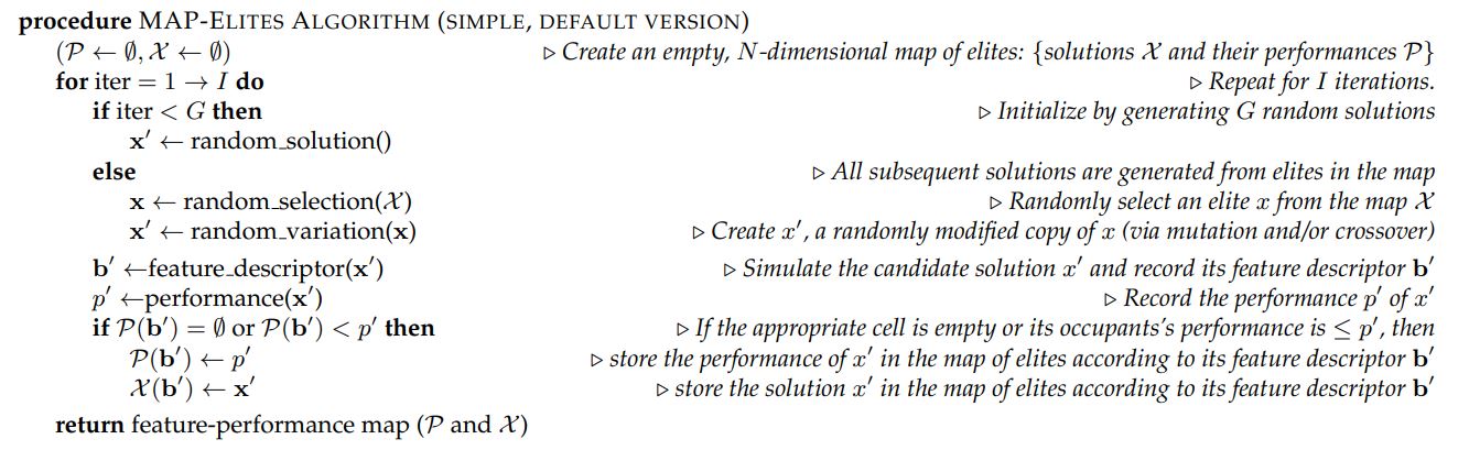
<p>Below is the general backbone of the MAP-Elites algorithm, taken from <em>Illuminating search spaces by mapping elites, Jean-Baptiste Mouret and Jeff Clune, 2015</em>.</p>

<p><img src="/assets/img/blog/map-elites.jpg" alt="MAP Elites" /></p>

<h2 id="discussion">Discussion</h2>

<h3 id="flexibility">Flexibility</h3>

<p>One important feature of the MAP-Elites is how flexible the algorithm is. Some of the things that we can tweak include</p>

<ul>
  <li><strong>Discretization:</strong> The granularity of the discretization is something that we control, based on the resources that are available. It could even be dynamic, we may want to gradually merge the cells so that in the end we are left with one solution that has the best performance.</li>
  <li><strong>Mutation:</strong> Following the traditional mutations in evolutionary optimization literature, vanilla MAP-Elites mutates the solutions by adding random noise to them. We could imagine other strategies for generating new solutions from the current set of elites. For instance, we could perform a cross-over operation over a number of the solutions, or perform several gradient ascent steps (when the objective is differentiable).</li>
  <li><strong>Behavior Space:</strong> The features that form the behavior space need not be hand-crafted. It may be possible to explicitly tune the behavior space and the feature descriptor function $b$ as the algorithm progresses.</li>
</ul>

<h3 id="map-elites-vs-optimization">MAP-Elites vs. Optimization</h3>

<p>Contrary to most ordinary optimization algorithms, MAP-Elites maintains a <em>population</em> of solutions. So, naturally, we need more memory to store the solutions (just imagine storing a large population of neural-nets with millions of parameters!). Why would we do that? What are some of the advantages that an illumination algorithm can bring to the table that might justify this additional computational overhead? To answer this question, we investigate several criteria that are used to evaluate optimization and illumination algorithms.</p>

<ol>
  <li><strong>Global Performance:</strong> The most basic criterion for evaluating the performance of any optimization algorithm is to measure the quality of the best solution found. Pure optimization algorithms generally yield better performing final results, which is expected as they are solely focused on maximizing $f$. However, in practice, MAP-Elites can find very good performing solutions and be competitive with traditional optimization algorithms. Because in MAP-Elites a larger portion of the search space is covered, the chances of stumbling upon a high-performing region in the search space gets higher.</li>
  <li><strong>Reliability:</strong> If we average the highest performing solution found for each cell in the behavior grid, across all runs and divide it by the best known performance in that cell, we get a measure of how reliable the algorithm is at finding good solutions with a particular behavior. This is an important performance measures for an illumination algorithm, as it indicates how clear is the picture of the behavior space that the algorithm gives us. Traditional optimization algorithms usually find high-performing solution but at the expense of coverage.</li>
  <li><strong>Coverage:</strong> The average number of cells in the behavior grid that a run of the algorithm is able to fill. Optimization algorithms usually perform much worse than illumination algorithms in this regard.</li>
</ol>

<p>Now, let’s see why we might want to encourage diversity. After all, the ultimate goal of optimization is to find a single highest-performing solution. There are several reasons why having a population of elites may be more desirable, albeit at the cost of consuming more memory.</p>

<ol>
  <li><strong>Robustness and Adaptation:</strong> When we have multiple good-enough solutions, each with different behaviors, we can get an ensemble of solutions that is much more robust to changes. Consider the racing robot example. If the racing environment suddenly becomes a bit more slippery, then the one high-performing solution may suddenly become completely obsolete. Whereas some other solution may now become optimal. Generally speaking, having multiple ways of solving a problem, gives us more ability to adapt when the environment changes.</li>
  <li><strong>Better Coverage $\rightarrow$ Better Optimization:</strong> MAP-Elites encourages exploration in different parts of the behavior space. This in itself could lead to finding high-performing regions in the search space. In the contrary, if an optimization algorithm starts out in a low-performing region, it is highly unlikely that it ever breaks free and explores other regions. This issue of getting stuck in local optima is something that all gradient-based optimization methods struggle with.</li>
  <li><strong>Performance-Behavior Relation:</strong> MAP-Elites illuminates the fitness potential of the whole behavior space, and not just the high-performing areas. This can potentially reveal relations between the performance and the dimensions of interest in the behavior space.</li>
  <li><strong>Diversity!:</strong> Finally, MAP-Elites allows us to create diversity in the dimensions of behavior that were chosen.</li>
</ol>]]></content><author><name></name></author><category term="blog" /><category term="Optimization" /><category term="Evolutionary" /><category term="QD" /><summary type="html"><![CDATA[An introduction to the algorithm.]]></summary></entry><entry><title type="html">Learning to Score Behaviors</title><link href="https://conflictednerd.github.io/blog/2022/Learning-to-Score-Behaviors/" rel="alternate" type="text/html" title="Learning to Score Behaviors" /><published>2022-09-21T14:52:46+00:00</published><updated>2022-09-21T14:52:46+00:00</updated><id>https://conflictednerd.github.io/blog/2022/Learning-to-Score-Behaviors</id><content type="html" xml:base="https://conflictednerd.github.io/blog/2022/Learning-to-Score-Behaviors/"><![CDATA[<p>(This is a note based on <a href="https://arxiv.org/abs/1906.04349">Learning to Score Behaviors for Guided Policy Optimization</a>. I am trying to expand and clarify some of the algorithms that were presented there. <span style="color:red">More content may be added to this note in the future!</span>)</p>

<p>The core question:</p>

<blockquote>
  <p>What is the right measure of similarity between two policies acting on the same underlaying MDP and how can we devise algorithms to leverage this information for RL?</p>
</blockquote>

<h2 id="concepts">Concepts</h2>

<h3 id="behavioral-embedding-map-bem">Behavioral Embedding Map (BEM)</h3>

<p>A function $\Phi:\Gamma \to \mathcal{E}$ that maps trajectories to embeddings. $\mathcal{E}$ can be seen as a behavioral manifold. Examples of BEMs include:</p>

<ol>
  <li>final state $\Phi (\tau) = s_H$,</li>
  <li>actions vector $\Phi(\tau) = [a_0, \cdots, a_H]$,</li>
  <li>total reward $\Phi(\tau) = \sum_{t=0}^{H}r_t$.</li>
</ol>

<h3 id="on-policy-policy-embedding">(On-Policy) Policy Embedding</h3>

<p>Given a policy $\pi$, let \(\mathbb{P}_\pi\) be the distribution it induces over the <em>space of trajectories, $\Gamma$</em>. For a behavioral embedding map $\Phi$, let \(\mathbb{P}_\pi^\Phi\) be the corresponding pushforward distribution on \(\mathcal{E}\) induced by $\Phi$. $P_\pi^\Phi$ is called the <em>policy embedding</em> of a policy $\pi$.</p>

<h3 id="wasserstein-distance">Wasserstein Distance</h3>

<p>Let $\mu, \nu$ be probability measures over \(\mathcal{X} \subseteq \mathbb{R}^m\), \(\mathcal{Y} \subseteq \mathbb{R}^n\) and let \(C: \mathcal{X}\times\mathcal{Y} \to \mathbb{R}\) be a cost function. For $\gamma &gt; 0$, a smoothed Wasserstein distance is defined as</p>

\[\mathrm{WD}_\gamma (\mu, \nu) := \min_{\pi \in \Pi(\mu, \nu)} \int_{\mathcal{X}\times\mathcal{Y}} C(\mathbf{x}, \mathbf{y})d_\pi(\mathbf{x}, \mathbf{y}) + \Sigma,\]

<p>where</p>

\[\Sigma = \gamma \mathrm{KL}(\pi \| \xi),\]

<p>$\Pi(\mu, \nu)$ is the space of couplings (joint distributions) over \(\mathcal{X}\times\mathcal{Y}\) with marginal distributions $\mu$ and $\nu$. When the cost is an $\mathscr{l}_p$ distance and \(\gamma = 0$, $\mathrm{WD}_\gamma\) is known as the Earth mover’s distance and the corresponding optimization is known as the <em>optimal transport problem</em>.</p>

<p>Notice that this is a hard optimization problem to solve: the search space is the space of couplings of $\mu, \nu$ and the objective involves an integral.</p>

<h3 id="wasserstein-distance-dual-formulation">Wasserstein Distance: Dual Formulation</h3>

<p>Let \(\mathcal{C}(\mathcal{X})\) and \(\mathcal{C}(\mathcal{Y})\) denote the space of continuous functions over \(\mathcal{X}\) and \(\mathcal{Y}\) respectively. We can view the cost function \(C: \mathcal{X}\times\mathcal{Y} \to \mathbb{R}\) as the <em>“ground cost”</em> of moving a unit of mass from $x$ to $y$. Using Fenchel duality, we can obtain the following dual formulation of the optimization problem that defines WD:</p>

\[\mathrm{WD}(\mu, \nu) = \max_{\lambda_\mu\in \mathcal{C}(\mathcal{X}), \lambda_\nu \in \mathcal{C}(\mathcal{Y})} \Psi(\lambda_\mu, \lambda_\nu),\]

<p>where</p>

\[\Psi(\lambda_\mu, \lambda_\nu) = \int_\mathcal{X} \lambda_\mu(\mathbf{x})d_\mu(\mathbf{x}) - \int_\mathcal{Y} \lambda_\nu(\mathbf{y})d_\nu(\mathbf{y}) - E_C(\lambda_\mu, \lambda_\nu).\]

<p>The last term, $E_C$ is known as the damping term and is defined as</p>

\[E_C (\lambda_\mu, \lambda_\nu) = \mathbb{I}(\gamma &gt; 0) \int_{\mathcal{X}\times\mathcal{Y}} \rho(\mathbf{x}, \mathbf{y}) d_\xi(\mathbf{x}, \mathbf{y}) + \mathbb{I}(\gamma = 0) \mathbb{I}(\mathcal{A}),\]

<p>for</p>

\[\rho(\mathbf{x}, \mathbf{y}) = \gamma \exp (\frac{\lambda_\mu(\mathbf{x}) - \lambda_\nu (\mathbf{y}) - C(\mathbf{x}, \mathbf{y})}{\gamma})\]

<p>and</p>

\[\mathcal{A} = \left[(\lambda_\mu, \lambda_\nu) \in \{(u, v) \mathrm{\\;s.t.\\;} \forall (\mathbf{x}, \mathbf{y}) \in \mathcal{X}\times\mathcal{Y}: u(\mathbf{x}) - v(\mathbf{y}) \leqslant C(\mathbf{x}, \mathbf{y})\}\right].\]

<p>We can set the damping distribution $d_\xi (\mathbf{x}, \mathbf{y})\propto 1$ for discrete domains and $d_\xi (\mathbf{x}, \mathbf{y}) = d_\mu(\mathbf{x})d_\nu(\mathbf{y})$ for continuous domains.</p>

<p>We have transformed the original optimization problem, but this new formulation now seems even more complicated! But note that if \(\lambda_\mu^{*}, \lambda_\nu^{*}\) are the functions achieving the maximum of $\Psi$, and $\gamma$ is sufficiently small, then \(\mathrm{WD}_\gamma(\mu, \nu) \approx \mathbb{E}_\mu[\lambda_\mu^{*}(\mathbf{x})] - \mathbb{E}_\nu[\lambda_\nu^{*}(\mathbf{y})]\), with equality when $\gamma = 0$.</p>

<p>For our purposes, we generally have \(\mathcal{X} = \mathcal{Y}\) and $C(x, x) = 0$ for all \(x\in \mathcal{X}\). Now if we let $\gamma = 0$, then one can see that \(\lambda_\mu^{*}(x) = \lambda_\nu^{*}(y) = \lambda^{*}(x)\) for all \(x\in\mathcal{X}\). In this case, \(\mathrm{WD}(\mu, \nu) = \mathbb{E}_\mu[\lambda^{*}(x)] - \mathbb{E}_\nu[\lambda^{*}(x)]\), which means that \(\lambda^{*}\) is a function that assigns high scores to regions where $\mu$ has more mass and low scores to those where $\nu$ has more mass. This means that we can interpret \(\lambda^{*}\) as a function that can distinguish policy embeddings of two policies. So, <strong>if we have \(\lambda^{*}\)</strong>, we can estimate \(\mathrm{WD}(\mu, \nu)\) by sampling from $\mu$ and $\nu$.</p>

<h3 id="computing-lambda_mu-and-lambda_nu">Computing \(\lambda_\mu^{*}\) and \(\lambda_\nu^{*}\)</h3>

<p>To make the optimization tractable, the paper uses RBF kernels and approximates them using random Fourier feature maps. As a result, the functions $\lambda$ that are learned have the following form</p>

\[\lambda(\mathbf x) = (\mathbf{p}^\lambda)^T\phi(\mathbf{x}),\]

<p>where $\phi$ is a random feature map with $m$ random features and $\mathbf{p}^\lambda \in \mathbb{R}^m$ are the parameters that we optimize. For RBF kernels, $\phi$ is defined as</p>

\[\phi(\mathbf{z}) = \frac{1}{\sqrt{m}}\cos(\mathbf{Gz}+\mathbf{b})\]

<p>for $\mathbf{z} \in \mathbb{R}^d$, where $\mathbf{G} \in \mathbb{R}^{m\times d}$ is a Gaussian with iid entries taken from \(\mathcal{N}(0, 1)\) and $\mathbf{b} \in \mathbb{R}^m$ has iid entries taken from $\mathrm{Uniform}(0, 2\pi)$. The $\cos$ function is applies elementwise.</p>

<p>From hereon, the optimization of $\Psi$ over $\lambda$ is synonymous with optimization over $\mathbf{p}^\lambda$. Having said these, we can optimize $\Psi$ by running SGD to find the optimal vectors $\mathbf{p}^{\lambda_\mu}, \mathbf{p}^{\lambda_\nu}$. Given kernels \(\kappa, \mathscr{l}\) and a fresh sample \((x_t, y_t) \sim \mu \otimes \nu\), the SGD step w.r.t. the current iterates $\mathbf{p}_{t-1}^\mu, \mathbf{p}_{t-1}^\nu$ satisfies:</p>

\[F(\mathbf{p}_1, \mathbf{p}_2, x, y) = \exp \left(\frac{\mathbf{p}_1^T \phi_\kappa(x) - \mathbf{p}_2^T \phi_\mathscr{l}(y) - C(x, y)}{\gamma}\right), \\\\
v_t = \frac{\alpha}{\sqrt{t}}\left(\phi_\kappa(x_t), -\phi_\mathscr{l} (y_t)\right)^T \\\\
\begin{pmatrix}
\mathbf{p}_{t+1}^\mu \\\\
\mathbf{p}_{t+1}^\nu
\end{pmatrix} =
\begin{pmatrix}
\mathbf{p}_{t}^\mu \\\\
\mathbf{p}_{t}^\nu
\end{pmatrix} + (1 - F(\mathbf{p}_t^\mu, \mathbf{p}_t^\nu, x_t, y_t))v_t.\]

<p>($\alpha$ is the learning rate)</p>

<p>In what comes next, these update equations are regarded as the <strong>BEM update step</strong>.</p>

<p>If \(\mathbf{p}^\mu_{*}, \mathbf{p}^\nu_{*}\) are the optimal dual vectors, \(\mathbf{p}_{*} = (\mathbf{p}^\mu_{*}, \mathbf{p}^\nu_{*})\), \((x_1, y_1), \cdots, (x_k, y_k) \stackrel{\mathrm{i.i.d.}}{\sim}\mu\otimes\nu\), \(\mathbf{v}_i^{\kappa, \mathscr{l}} = (\phi_\kappa(x_i), -\phi_\mathscr{l} (y_i))\) for all $i$, and $\hat{\mathbb{E}}$ denotes the empirical expectation over the $k$ samples, then we can get an estimate of $\mathrm{WD}_\gamma (\mu, \nu)$ as</p>

\[\widehat{\mathrm{WD}}_\gamma(\mu, \nu) = \hat{\mathbb{E}} \left[\left&lt;\mathbf{p}_{*}, \mathbf{v}_i^{\kappa, \mathscr{l}} \right&gt; - \frac{F(\mathbf{p}^\mu_{*}, \mathbf{p}^\nu_{*}, x_i, y_i)}{\gamma}\right]\]

<p>To put things into perspective, if $\pi_1, \pi_2$ are two policies and $\Phi$ is a behavioral embedding map, we can write</p>

\[\mathrm{WD}_\gamma (\mathbb{P}_{\pi_1}^\Phi, \mathbb{P}_{\pi_2}^\Phi) \approx \mathbb{E}_{\tau\sim\mathbb{P}_{\pi_1}}[\lambda_1^{*}(\Phi(\tau))] - \mathbb{E}_{\tau\sim\mathbb{P}_{\pi_2}}[\lambda_2^{*}(\Phi(\tau))]\]

<p>with \(\lambda_1^{*}, \lambda_2^{*}\) being the optimal dual functions. The maps \(s_i := \lambda_i^{*} \circ \Phi : \Gamma \to \mathbb{R}\) define score functions over the space of trajectories, and if $\gamma$ is close to zero, they assign higher scores tot trajectories from $\pi_i$ whose behavior embedding is common under $\pi_i$ but uncommon under $\pi_{j\neq i}$.</p>

<h2 id="algorithms">Algorithms</h2>

<h3 id="random-features-wasserstein-sgd-algorithm-1">Random Features Wasserstein SGD (Algorithm 1)</h3>

<ol>
  <li><strong>Input:</strong> kernels \(\kappa, \mathscr{l}$ over $\mathcal{X}, \mathcal{Y}\) respectively, with corresponding random feature maps \(\phi_\kappa, \phi_\mathscr{l}\), smoothing parameter $\gamma$, step size $\alpha$, number of optimization rounds $M$, initial dual vectors \(\mathbf{p}_0^\mu, \mathbf{p}_0^\nu\).</li>
  <li>for $t = 0, \cdots, M$ :
    <ol>
      <li>Sample $(x_t, y_t) \sim \mu \otimes \nu$.</li>
      <li>Update \(\begin{pmatrix}\mathbf{p}_{t}^\mu \\ \\ \mathbf{p}_{t}^\nu\end{pmatrix}\) using <strong>BEM update step</strong>.</li>
    </ol>
  </li>
  <li><strong>Return:</strong> $\mathbf{p}_M^\mu, \mathbf{p}_M^\nu$.</li>
</ol>

<p><strong>How does this work in practice?</strong> Let’s say we have a base policy $b$ and another policy $\pi$ and we want to estimate \(\mathrm{WD}_\gamma (\mathbb{P}_b^\Phi, \mathbb{P}_\pi^\Phi)\). Note that these can be random variables; for instance, $b$ might be chosen uniformly from a set of policies $B = \{b_1, \cdots, b_n\}$. First, we need to choose a behavior embedding map $\Phi: \Gamma \to \mathbb{R}^d$ that maps trajectories into $d$ dimensional vectors. Then, we must initialize random feature maps \(\phi_b, \phi_\pi: \mathbb{R}^d \to \mathbb{R}^m\) that map the outputs of $\Phi$ to $\mathbb{R}^m$. From what I understood from the code, we can use a single random feature map for both $b$ and $\pi$. Assuming this is the case, we essentially need to initialize \(\phi(\mathbf{z}) = \frac{1}{\sqrt m} \cos (\mathbf{Gz} + \mathbf{b})\). To do so, we sample \(\mathbf{G} \in \mathbb{R}^{m\times d}\) from \(\mathcal{N}(0, 1)\) and $\mathbf{b} \in \mathbb{R}^m$ from $\mathrm{Uniform}(0, 2\pi)$. Next, we initialize dual parameter vectors $\mathbf{p}^\pi, \mathbf{p}^b$ that will be optimized. Finally, we need to run $\pi$ and $b$ to obtain $k$ sample trajectories. These trajectories are saved in buffers $B_\pi, B_b$. (Actually, we only need the behavior embedding of the trajectories, i.e., $\Phi(\tau)$s). The last step is to run SGD to find optimal parameters \(\mathbf{p}_{*}^\pi, \mathbf{p}_{*}^b\). This is done using the algorithm presented above, where sampling $(x_t, y_t) \sim \mu \otimes\nu$ is analogues to sampling from the buffers.</p>

<p>When all is set and done, we have \(\mathbf{p}_{*}^\pi, \mathbf{p}_{*}^b\) and we can write</p>

\[\widehat{\mathrm{WD}}_\gamma(\mathbb{P}_b^\Phi, \mathbb{P}_\pi^\Phi) = \frac{1}{k}\sum_{i=1}^{k} \left&lt;\mathbf{p}_{*}, \mathbf{v}_i\right&gt; - \frac{F(\mathbf{p}^b_{*}, \mathbf{p}^\pi_{*}, x_i, y_i)}{\gamma}\]

<p>where $x_i \in B_b$, $y_i \in B_\pi$ and $F$, $\mathbf{v}_i$ are as were defined in the previous section.</p>

<p>Additionally, we we can get the following score function that assigns high scores to trajectories that are similar to $\pi$ but different from $b$:</p>

\[s_\pi (\tau) = \lambda_\pi^{*}  \circ \Phi (\tau) = \frac{1}{\sqrt{m}}(\mathbf{p}_{*}^\pi)^T\cos(\mathbf{G}(\Phi(\tau))+ \mathbf{b})\]

<p><strong>Implementation detail:</strong> In the released code, $\gamma = 1$ is chosen.</p>

<h3 id="a-simple-behavior-guided-algorithm-algorithm-2">A Simple Behavior-Guided Algorithm (Algorithm 2)</h3>

<p>Now, let’s see how we can use the behavior functions to devise a simple algorithm.</p>

<p>Imagine a simple scenario in which we have a policy $b$ for doing some task $T_1$ and we want to find a policy $\pi_\theta$ for solving another task $T_2$ that exhibits similar behavior to $b$. The idea is to use the regular reward for task $T_2$ to optimize $\theta$, but also use the scoring functions that were found in the previous section to encourage trajectories with similar behavior to $b$.</p>

<h4 id="learnable-parameters">Learnable parameters</h4>

<ol>
  <li>parameters of our policy $\theta_0$.</li>
  <li>parameters of behavioral test function $\mathbf{p}^b, \mathbf{p}^{\pi_{\theta_0}} \in \mathbb{R}^m$</li>
</ol>

<h4 id="initializations">Initializations</h4>

<ol>
  <li>behavioral embedding map $\Phi:\Gamma \to \mathbb{R}^d$ to encode trajectories</li>
  <li>random kernels $\mathbf{G} \in \mathbb{R}^{m\times d}$ from normal distribution and $\mathbf{b} \in \mathbb{R}^m$ from uniform distribution</li>
  <li>buffers $B_b, B_\pi$ for storing trajectories</li>
</ol>

<h4 id="hyperparameters">Hyperparameters</h4>

<ol>
  <li>weighting coefficient $\beta \geqslant 0$ and smoothing coefficient $\gamma &gt; 0$</li>
  <li>number of iterations $T$ and rollouts per iteration $M$</li>
  <li>learning rates $\alpha$ for behavioral test functions and $\eta$ for policy optimization</li>
</ol>

<h4 id="algorithm">Algorithm</h4>

<ol>
  <li>for $t = 1, \cdots, T$:
    <ol>
      <li>Collect trajectories $\{\tau_i^\pi\}_{i=1}^M$ using policy \(\pi_{t-1} = \pi_{\theta_{t-1}}\) and add them to the buffer \(B_\pi\)</li>
      <li>Collect trajectories $\{\tau_i^b\}_{i=1}^M$ using policy $b$ and add them to the buffer $B_b$</li>
      <li>Update behavioral test functions $\lambda_\pi, \lambda_b$ with <em>Random Features Wasserstein SGD</em></li>
      <li>Optimize the policy by taking SGA step \(\theta_t = \theta_{t-1} + \eta \hat\nabla_\theta \hat F(\theta_{t-1})\)</li>
      <li>Clear the buffers</li>
    </ol>
  </li>
</ol>

<h4 id="implementation-details">Implementation details</h4>

<ol>
  <li>
    <p>The objective function $F(\theta)$ that policies perform SGA over is of the form</p>

\[F(\theta) = \mathbb{E}_{\tau_1, \tau_2 \sim \mathbb{P}_{\pi_{t-1}} \otimes \mathbb{P}_b} \left[\hat R(\tau_1, \tau_2)\right]\]

    <p>where $\hat R (\tau_1, \tau_2)$ is the surrogate reward defined as</p>

\[\hat R (\tau_1, \tau_2) = \sum_i \frac{\pi_{\theta}(a_i \mid s_i)}{\pi_{t-1}(a_i \mid s_i)}A^{\pi_{t-1}} (s_i, a_i) - \beta\widehat{\mathrm{WD}}_\gamma (\mathbb{P}_{\pi_\theta}^{\Phi}, \mathbb{P}_b^\Phi).\]

    <p>The first summation term is the regular advantage weighted by importance sampling ratios that is used in regular policy optimization algorithms. The second term, involving Wasserstein distance is what encourages behaviors similar to $b$. Using the estimates of WD we can write</p>

\[F(\theta) \approx \mathbb {E}_{\tau \sim \mathbb{P}_{\pi_\theta}}\left[\mathcal{R}(\tau) - \beta \lambda_{\pi_\theta}^{*}(\Phi(\tau))\right] + \beta \mathbb{E}_{\tau \sim \mathbb{P}_b} \left[\lambda_b^{*}(\Phi(\tau))\right].\]

    <p>Consequently,</p>

\[\nabla_\theta F(\theta) \approx \nabla_\theta \mathbb{E}_{\tau\sim \mathbb{P}_{\pi_\theta}}[\mathcal{R}(\tau)] - \beta \nabla_\theta\mathbb{E}_{\tau\sim \mathbb{P}_{\pi_\theta}}[\lambda_{\pi_\theta}^{*}(\Phi(\tau))]\]

    <p>The first term is the regular policy gradient and <em>the second term can be considered as a constant reward</em> that is added to each trajectory based on its similarity to the the behavior of $\pi_\theta$ and its dissimilarity to the behavior of $b$.</p>

    <p><strong>So, to optimize $F$ all we need to do is to add a reward of \(-\beta \lambda_{\pi_\theta}^{*}(\Phi(\tau))\) to each transition in the trajectory $\tau$.</strong></p>
  </li>
  <li>
    <p>Because the base policy $b$ is fixed, we can append trajectories into its buffer $B_b$ without resetting it.</p>
  </li>
  <li>
    <p>In the third step where we update behavioral test function parameters $\mathbf{p}$, we can start the optimization from the previously found parameters which may help speed up the convergence.</p>
  </li>
  <li>
    <p>In the paper, the authors suggest that we first optimize the policy ($F$) and then optimize behavioral test functions ($\lambda$), which is strange to me.</p>
  </li>
</ol>]]></content><author><name></name></author><category term="blog" /><category term="RL" /><category term="paper-summary" /><summary type="html"><![CDATA[A summary of the paper.]]></summary></entry><entry><title type="html">Optimization Primer</title><link href="https://conflictednerd.github.io/blog/2022/Optimization-Primer/" rel="alternate" type="text/html" title="Optimization Primer" /><published>2022-08-27T01:54:49+00:00</published><updated>2022-08-27T01:54:49+00:00</updated><id>https://conflictednerd.github.io/blog/2022/Optimization-Primer</id><content type="html" xml:base="https://conflictednerd.github.io/blog/2022/Optimization-Primer/"><![CDATA[<p>(Based on <a href="https://youtu.be/NSd6zOKZkpI">a lecture</a> by professor Coralia Cartis, University of Oxford)<br />
(I don’t currently plan to extend it, but may expand and add more details to some of the later chapters in the future. I also like to eventually add some useful resources (books, talks, notes, etc.) about optimization)</p>

<p>This brief note is about optimization problems. Though the main focus is on the general non-convex optimization problem, a lot of the methods borrow some ideas from convex optimization, so there are a lot of similarities. Generally, different approaches to solving these problems can be put into three main categories:</p>
<ol>
  <li>Those that use derivatives, be it first order (gradient descent) or higher order (Newton’s method),</li>
  <li>Those that don’t use derivatives, regarded as derivative-free methods (evolutionary methods),</li>
  <li>Inexact and probabilistic methods.</li>
</ol>

<p>The first two are covered in this post. Also, for derivative-free methods, only unconstrained problems are considered.</p>

<h1 id="introduction">Introduction</h1>

<h2 id="the-optimization-problem">The Optimization Problem</h2>

<p>In its most general form, an optimization problem has the following form:</p>

\[\mathrm{minimize}\;\; f(x) \;\;\mathrm{subject\;to} \;\; x \in \Omega \subseteq \mathbb{R}^n.\]

<p>Furthermore, the following assumptions commonly hold:</p>

<ul>
  <li>$f: \Omega \to \mathbb{R}$ is a smooth function,</li>
  <li>The feasible set, $\Omega$, is defined by <strong>finitely many</strong> smooth constraints.</li>
</ul>

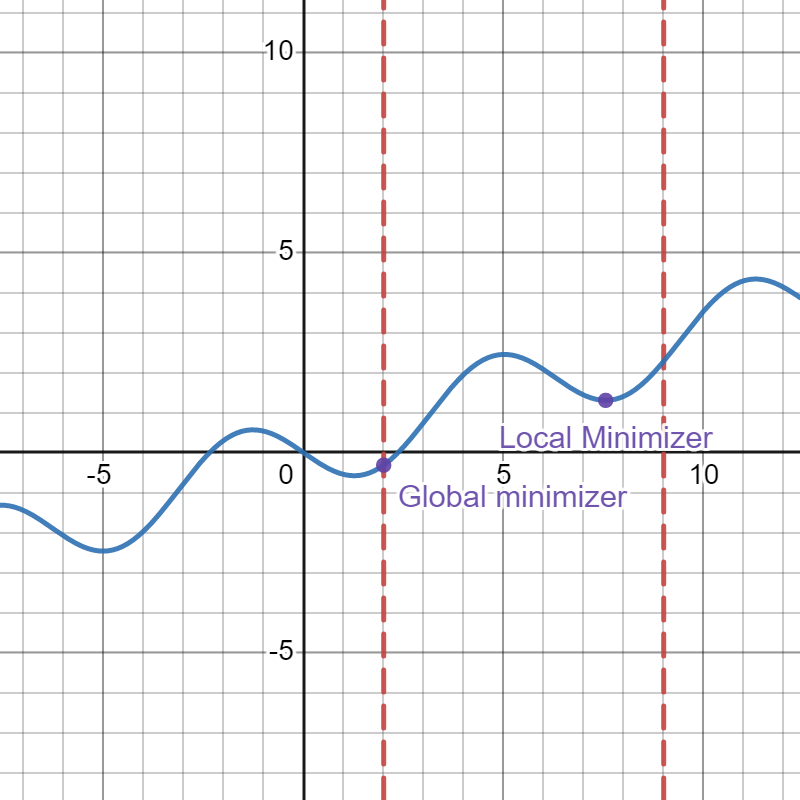
<p>The solution to this problem is a point \(x^{*}  \in \Omega\) in which $f$ attains its minimum value. We are sometimes also interested in <em>local minimizers</em>; these are points such as \(x^{*} \in \Omega\) for which a neighborhood \(\mathcal{N} (x^{*}, \delta)\) exists such that \(f(x) \geqslant f(x^{*})\) for all \(x \in \Omega \cap \mathcal{N}(x^{*}, \delta)\).<br />
In the figure below, you can see the function $f$ (blue) is constrained to the closed interval between the red lines. You can see a local and global minimizer for $f$ in the feasible set.</p>

<div class="text-center">
  <img src="/assets/img/blog/optima.png" class="img-fluid" style="max-width: 70%;" />
</div>

<h2 id="linear-and-quadratic-optimization">Linear and Quadratic Optimization</h2>

<p>Two simple, yet important special cases of the optimization problem are linear and quadratic optimization.<br />
In linear optimization (programming), the objective function $f$ and the constraints that define $\Omega$ are all linear functions. So, a linear optimization problem has the following form:</p>

\[\min_{x\in \mathbb{R}^n} c^Tx \;\; \mathrm{subject\; to} \\
a_i^Tx = b_i, \;\;\; \forall i \in I, \\
a_j^Tx\geqslant b_j \;\;\; \forall j \in J.\]

<p>Quadratic programming is similar in that the constraints are linear, but the objective function becomes quadratic:</p>

\[\min_{x\in \mathbb{R}^n} c^Tx + \frac{1}{2}x^THx \;\; \mathrm{subject\; to} \\
a_i^Tx = b_i, \;\;\; \forall i \in I, \\
a_j^Tx\geqslant b_j \;\;\; \forall j \in J.\]

<h2 id="solutions-and-derivatives">Solutions and Derivatives</h2>

<p>Before talking about the algorithms for solving optimization problem, it is useful to see the relation between minimizers and the derivatives. In a nutshell, this section is trying to generalize the simple idea of <em>“a minimizer is where the derivative is zero and the second derivative is positive”</em> that we know from single-variable calculus.</p>

<p>Notice that in this section we are concerned with <u>unconstrained problems</u>. Optimality conditions for constrained problems are more complicated, though they make use of some of these ideas. We will briefly talk about optimality conditions for constrained problems in another section.</p>

<h3 id="first-order-optimality-condition">First Order Optimality Condition</h3>

<p><strong>Theorem:</strong> Suppose</p>

\[f \in
\mathcal{C}
^1(\mathbb{R}^n)\]

<p>(it’s differentiable with a smooth derivative) and that \(x^{*}\) is a local minimizer of $f$. Then, \(x^{*}\) is a stationary point for $f$, i.e., the gradient of $f$ at \(x^{*}\) is zero.</p>

\[x^{*} \mathrm{\;is\;local\;minimizer\;of\;} f \implies \nabla f (x^{*} ) = 0.\]

<p><strong>An Aside:</strong> Remember that $\nabla f (x) = [\frac{\partial f}{\partial x_1}(x), \cdots,\frac{\partial f}{\partial x_n}(x)]^T$.</p>

<h3 id="second-order-optimality-condition">Second Order Optimality Condition</h3>

<p>Not all stationary points are minimizers. A stationary point may be a saddle point or even a maximizer! So, we need to add some other condition if we are to distinguish minimizers from other types of stationary points. The second order necessary condition gives us precisely this.</p>

<p><strong>Theorem:</strong> Suppose $f\in \mathcal{C}^{2} (\mathbb{R}^{n})$ and that \(x^{*}\) is a local minimizer of $f$. Then, \(\nabla^{2} f(x^{*})\) is <u>positive-semidefinite</u>.</p>

<p>We also have a second order sufficient condition:</p>

<p><strong>Theorem:</strong> Suppose $f\in \mathcal{C}^2(\mathbb{R}^n)$ and that \(x^{*} \in \mathbb{R}^n\) is such that \(\nabla f(x^{*} ) = 0\) and \(\nabla^2f(x^{*})\) is <u>positive-definite</u>. Then, \(x^{*}\) is surely a local minimizer of $f$.</p>

<p><strong>An Aside:</strong> Remember that $\nabla^2f(x)$ is a matrix, called the <em>Hessian</em>, defined as</p>

\[\nabla^2 f(x) =
\begin{bmatrix}
&amp;\frac{\partial^2 f}{\partial x_1^2}(x), \cdots, &amp;\frac{\partial^2 f}{\partial x_1\partial x_n}(x) \\
&amp;\vdots \ddots &amp;\vdots \\
&amp;\frac{\partial^2 f}{\partial x_n \partial x_1}(x), \cdots, &amp;\frac{\partial^2 f}{\partial x_n^2}(x)
\end{bmatrix}.\]

<p>Notice that the Hessian matrix is always symmetric. This is particularly convenient, as it means that the Hessian is diagonalizable and its eigenvectors can be chosen to be orthonormal.</p>

<p><strong>Another Aside:</strong> Remember that a <u>symmetric</u> matrix $M$ is called positive-definite if for all vectors $x\in \mathbb{R}^n \backslash \{0 \}$, we have $x^TMx &gt; 0$. Similarly, $M$ is positive-semidefinite if $x^TMx \geqslant 0$.<br />
Alternatively, we could say that $M$ is positive-definite iff all its eigenvalues are positive and it is positive-semidefinite iff all its eigenvalues are non-negative. It is often useful to think of definiteness like this, in terms of eigenvalues.</p>

<p>Now let’s revisit the second order optimality conditions. A stationary point can be a (local) minimizer only if the Hessian at that point is positive-semidefinite (necessary condition). However, if the Hessian is positive-definite, we can be certain that the point is a minimizer (sufficient condition).</p>

<h2 id="finding-derivatives">Finding Derivatives</h2>

<p>Many of the methods that we will discuss rely on derivatives (and sometimes Hessians). Therefore, it is nice to understand how we might provide derivatives to solvers before discussing the methods themselves. When the objective and the constraints are simple, we can of course compute their derivatives by hand and write code that explicitly computes gradients at each point. But often, this is not possible and we have to calculate (or approximate) derivatives automatically. There are several methods to do this:</p>
<ol>
  <li><strong>Automatic Differentiation:</strong> These methods break down the code that <em>evaluates</em> $f$ into elementary arithmetic operations and compute the derivatives using chain rule. Think of modern deep learning frameworks such as PyTorch, TensroFlow, JAX.</li>
  <li><strong>Symbolic Differentiation:</strong> These methods can be thought of as an extension to the differentiate-by-hand method. They manipulate the algebraic expression of $f$ (when available) and compute the derivative. Think of symbolic packages of MAPLE, MATLAB, MATHEMATICA.</li>
  <li><strong>Finite Differences:</strong> When we expect $f$ to be smooth and without much noise, finite differences methods can be used to approximate the gradients. When we don’t have an nicely formed expression for evaluating $f$, but nevertheless can evaluate it efficiently (e.g., evaluation may involve running a simulation) we can use these methods.</li>
</ol>

<h1 id="unconstrained-optimization">Unconstrained Optimization</h1>

<h2 id="generic-method">Generic Method</h2>

<p>Consider the problem of minimizing a function $f$ over the $\mathbb{R}^n$. In derivative-based methods that are discussed below, we assume $f\in \mathcal{C}^1(\mathbb{R}^n)$ or $f\in \mathcal{C}^2(\mathbb{R}^n)$.</p>

<p>We start by a very generic iterative method:</p>

<pre><code class="language-pseudocode">Generic Method(GM):
    Start with an initial guess 𝑥₀.
    while Termination criteria not reached:
        Compute a change vector 𝑣 based on the previous guess and the data
        𝑥ₖ₊₁ = 𝑥ₖ + 𝑣
        𝑘 = 𝑘 + 1
</code></pre>

<p>Now by filling in the gaps we can get different algorithms.</p>

<ol>
  <li><strong>Termination Criteria:</strong> The most often used stopping condition is to check if the gradient has become too small, i.e., $\|\nabla f(x_k)\|&lt;\epsilon$ along with the decreasing property, i.e., $f(x_{k+1}) &lt; f(x_k)$. But we can also use some more complicated eigenvalue-based criteria as well. In most cases though, we just check the norm of the gradient.</li>
  <li><strong>Computing The Change Vector:</strong> This is where the most variation in algorithms can be seen. How are we to find a vector $v$  following which allows us to further minimize the value of $f$? There are different approaches to finding this vector (line-search, trust region) that will be discussed below. But, at the heart of all these methods is a simple idea: we can use a simple, local model $m_k$ to approximate $f$ around $x_k$, and then try to minimize $m_k$. When we have access to derivatives, we can choose $m_k$ to be a <em>linear</em> or <em>quadratic</em> function based on the Taylor expansion of $f$. Of course this approximation will not work great if we move too far away from $x_k$, so we have to take that into consideration when computing $v$.</li>
</ol>

<p>Before presenting any concrete algorithms, it is useful to mention some desirable properties that we would like to have in an iterative algorithm. Ideally, we want to our algorithm to <strong>converge globally</strong>, meaning that the algorithm converges and terminates, regardless of the starting point (not to be confused with convergence to global minima!). If that is not possible, we would like to have some <strong>local convergence</strong> guarantee, meaning that the algorithm converges to a local minimizer or stationary point when we start sufficiently close to one. One final consideration is the <strong>speed of convergence</strong>. We would like to have algorithms that not only converge, but do so quickly!</p>

<p>With these considerations in mind, we proceed to give the first algorithms for solving the optimization problem, based on the general recipe of the Generic Method.</p>

<h2 id="line-search-methods">Line-search Methods</h2>

<p>Line-search methods work by first finding a descent direction $s_k\in\mathbb{R}^n$, and then computing a step size $\alpha_k&gt;0$ such that $f(x_k + \alpha_k s_k) &lt; f(x_k)$.</p>

<p><strong>Descent Direction:</strong> A descent direction is a vector $s_k$ that if we take a sufficiently small step in its direction, will take us to a point where the value of $f$ is smaller. $-\nabla f(x_k)$ is one such direction that we can use. Generally speaking, any vector $s_k$ that satisfies $\nabla f(x_k)^T s_k &lt; 0$ is a descent direction (Think of directional derivatives!).</p>

<p><strong>Step Size:</strong> Given a direction $s_k$, we now have to compute a step-size $\alpha_k&gt;0$ along $s_k$ such that</p>

\[f(x_k + \alpha_k s_k) &lt; f(x_k).\]

<p>Because $s_k$ is a descent direction, we know that a very small step size will satisfy the above inequality. But we also want the step size to be as large as possible, so that we converge faster. Fundamentally, line-search is a method for selecting an appropriate step size. So, we will first discuss the line-search methods for finding good step-sizes, and then talk about the choice of the descent direction (steepest descent is not always the best choice!).</p>

<h3 id="exact-line-search">Exact Line-search</h3>

<p>Exact line-search finds the optimal step-size by solving an inner single-variable optimization</p>

\[\alpha_k = \arg \min_{\alpha&gt;0} f(x_k + \alpha s_k).\]

<p>This step size is optimal in the sense that $\alpha_k s_k$ is the most decreasing step we can take in the direction of $s_k$. Additionally, this is a single variable optimization (the only variable is $\alpha$) which is easier to solve than the full optimization that we had before. Unfortunately, repeatedly solving this inner optimization is computationally expensive for non-linear objectives.</p>

<p><strong>An Aside:</strong> Conceptually, think of exact line-search as a method that shrinks the search space from $\mathbb{R}^n$ to a single line. What the full exact line-search does is finding a promising line in $\mathbb{R}^n$ and searching along it to find a better solution.</p>

<h3 id="inexact-line-search">Inexact Line-search</h3>

<p>Inexact line-search uses an step-size that may not be optimal, but is “good enough”, i.e., taking a step of that size will decrease $f$ by a “sufficient amount”, proportional to $\alpha_k$ and $\nabla f(x_k)^Ts_k$.</p>

<p>One way of defining this sufficient amount is by using the <strong>Armijo condition</strong>. Let $\Phi_k (\alpha) := f(x_k + \alpha s_k)$. The Armijo condition requires that</p>

\[\Phi_k(\alpha_k) \leqslant y_\beta(\alpha_k) := \Phi_k(0) + \beta\alpha_k\Phi'(0),\]

<p>for some $\beta \in (0, 1)$.</p>

<p>An algorithm that uses the Armijo condition will start with some large, initial step size $\alpha_k$, and backtracks (binary search style!) to find an $\alpha_k$ that satisfies the above condition. (<em>What should the initial step size be? Sometimes we just start with 1 agnostically, but there are some very interesting methods for “guessing” a good starting value!</em>)</p>

<p><strong>Intuitively, what is the Armijo condition doing?</strong> Like the exact line-search, we are restricting $f$ to a line defined by the direction of $s_k$. This restricted version is $\Phi_k$. Exact line-search minimizes $\Phi_k$. However, here we are finding the line that is tangent to $\Phi_k$ at $0$, rotate it upwards by a small amount determined by $\beta$, and just find any point that is below this rotated line. The more we rotate the tangent, the easier it will be to find a point that lies below it, but also the more inaccurate (and suboptimal) the resulting step size may be.</p>

<p>The figure below may be helpful to better understand this. Notice that $\Phi(\alpha)$ is the restricted version of $f$, $y_1(\alpha)$ is the tangent to it at zero, and $y_{0.6}(\alpha)$ is its the rotated version. Selecting any point at which $\Phi$ is below this line will result in a “sufficiently good” step size.</p>

<div class="text-center">
  <img src="/assets/img/blog/armijo.jpg" class="img-fluid" style="max-width: 70%;" />
</div>

<h3 id="steepest-descent">Steepest Descent</h3>

<p>Choosing $s_k$ to be the negative gradient and using any line-search method will give an algorithm that is often called the <strong>method of steepest descent</strong>. Notice that the line-search, be it exact or with Armijo-like conditions, is key here, as it allows us to show some nice convergence properties. The next theorem, showcases this.</p>

<p><strong>Theorem:</strong> Let $f$ be sufficiently smooth (i.e., $\nabla f$ is Lipschitz continuous) and bounded from below. The method of steepest descent globally converges, meaning that</p>

\[\|\nabla f(x_k)\| \to 0 \;\; \mathrm{as} \;\; k \to \infty.\]

<p>Although steepest descent (SD) converges, it does so slowly. This is because SD is scale-dependent. Look at the Contour plots below and the evolution of the SD solution. In the first plot, SD (exact line-search) is able to find the minimizer in one step. However, if the problem becomes slightly ill-conditioned, as is in the second plot, it will take much longer for SD to converge.</p>

<p><img src="/assets/img/blog/sd1.png" style="zoom:20%;" /><img src="/assets/img/blog/sd2.png" style="zoom:20%;" /></p>

<p><strong>An Aside:</strong> SD converges linearly and the condition number of the Hessian matrix determines the rate of convergence for SD. This highlights the issue with SD: because it doesn’t take the curvature (Hessian) into account, it may perform poorly. As can be seen in the plots above, taking the direction of steepest descent is not always the best choice.</p>

<h3 id="beyond-steepest-descent">Beyond Steepest Descent</h3>

<p>As we saw, SD with line-search can have very slow convergence rates. The simplest way for dealing with the ill-conditioning that was mentioned is to simply scale our variables (batch normalization in neural nets claims to be doing this!). Second order methods, headlined by the famous Newton’s method, use the Hessian (or an approximation of it) to automatically address this issue. In this section, general ideas behind these methods are presented without going into much details about the specificities of the algorithms.</p>

<h4 id="newtons-method">Newton’s Method</h4>

<p>Let’s revisit how we ended up with $-\nabla f(x_k)$ as the descent direction. In essence, we approximated $f$ near $x_k$ with a linear model. Using the Taylor expansion, this linear model was</p>

\[m_k(s) = f(x_k) + \nabla f(x_k)^T s.\]

<p>Now, if we want to minimize this function (subject to $\|s\| = \|\nabla f(x_k)\|$ to bound the values from below), we should let $s=-\nabla f(x_k)$. Therefore, the negative gradient direction was selected as the direction that minimizes the local linear model that we chose for $f$.</p>

<p>The idea behind Newton’s method is to use a second order approximation to $f$. Suppose $B_k$ is a symmetric positive-definite matrix and that we choose to locally approximate $f$ by</p>

\[m_k(s) = f(x_k) + \nabla f(x_k)^T s +\frac{1}{2}s^TB_ks.\]

<p>Because $B_k$ is positive-definite, this quadratic function has a unique minimum that can be found by:</p>

\[\nabla_s m_k(s^{*} ) = 0 \implies -\nabla f(x_k) = B_ks^{*} .\]

<p>So, to find the direction of descent we must solve this system of linear equations for $s^{*} $.</p>

<p>One question remains, how should we choose $B_k$? First, notice that we need $B_k$ to be positive-definite to guarantee that $s^{*}$ is a descent direction:</p>

\[s^T\nabla f(x_k) &lt; 0 \implies -s^TB_ks &lt; 0 \implies s^TB_ks &gt;0.\]

<p>If $\nabla^2 f(x_k)$ is positive-definite, we can let $B_k = \nabla^2 f(x_k)$ as this would result in the best quadratic approximation of $f$ (Taylor expansion). This choice gives raise to an algorithm known as the <em>damped Newton method</em>.</p>

<p>However, the Hessian need not be positive-definite, it may be that its positive-semidefinite. So this choice of $B_k$ requires $f$ to be locally strictly convex everywhere! Even if this is the case, we still need a number of additional assumptions to prove global convergence. To summarize, Newton’s method</p>

<ul>
  <li>is scale-invariant (solves the issue with steepest descent),</li>
  <li>can speed up convergence (quadratic convergence) for functions with positive-definite Hessians,</li>
  <li>has no global convergence guarantees, even worse, it may not converge at all for some simple examples.</li>
</ul>

<h4 id="modified-newton-method">Modified Newton Method</h4>

<p>When the Hessian is not positive-definite, we can “perturb” it a little so that it becomes sufficiently positive definite. In modified Newton method the descent direction is found by solving a slightly different system of linear equaitons:</p>

\[(\nabla^2 f(x_k) + M_k)s_k = -\nabla f(x_k),\]

<p>where $M_k$ is chosen such that $\nabla^2 f(x_k) + M_k$ is “sufficiently” positive-definite. Here, we will not get into the details of computing $M_k$.</p>

<p>This allows Newton’s method to be used with general objectives that don’t necessarily have positive-definite Hessians. However, we still need some additional assumptions to guarantee their global convergence.</p>

<h4 id="quasi-newton-methods">Quasi-Newton Methods</h4>

<p>When we don’t have access to second order derivatives, we can use a class of methods called quasi-Newton methods, to compute an approximation of the Hessian, $B_k \approx \nabla^2 f(x_k)$. A very general description of these methods is as follows: we start by an initial guess, $B_0$. After computing $s_k$ by solving $B_ks_k = -\nabla f(x_k)$ and setting $x_{k+1} = x_k + \alpha_ks_k$, we compute a (cheap) update $B_{k+1}$ of $B_k$.</p>

<p>Again, we don’t go into the details of how $B_k$ is updated. There are several methods that use this idea. BFGS and DFP are two of the most important ones that are considered to be state-of-the-art for unconstrained optimization.</p>

<p>Quasi-Newton methods are faster than Newton’s method, they require $\mathcal{O}(n^2)$ calculations per iteration as opposed to the $\mathcal{O}(n^3)$ required by Newton’s method. They also converge faster (in fewer iterations) compared to steepest descent methods, as they leverage curvature information.</p>

<h3 id="line-search-wrap-up">Line-search Wrap-up</h3>

<p>In this final section, let’s put all the things that we saw about line-search together so that we can have a clear idea of what line-search methods are doing.</p>

<p>At the $k$-th step, line-search methods locally approximate the non-convex objective function $f$ with a simple model $m_k$. This model can be linear, in which case it has the form $m_k(s) = f(x_k) + \nabla f(x_k)^Ts$ or quadratic, in which case it has the form $m_k(s) = f(x_k) + \nabla f(x_k)^Ts + \frac{1}{2}s^TB_k s$. When we have access to the Hessian, we can use $B_k = \nabla^2 f(x_k)$, otherwise, we can use estimates of the Hessian.</p>

<p>Once we have this model $m_k$, we use it to find a descent direction, $s_k$. This direction is found by minimizing the model, $m_k$. In the case of a linear model, this direction is $-\nabla f(x_k)$ and in the case of the quadratic model it is the solution to $B_ks_k = -\nabla f(x_k)$. Notice two important points:</p>

<ul>
  <li>When we use a linear model, $m_k$ is not bounded from below. Therefore, we can’t minimize it. To address this issue, we actually solve the constrained optimization $\min_{s}m_k(s)$ subject to $\|s\|&lt;\nabla f(x_k)$.</li>
  <li>When we use a quadratic model, $m_k$ is not bounded from below unless it is a convex, which is the case if and only if $B_k$ is positive-definite. So, when $B_k$ is not positive-definite, we perturb it. In essence, we locally approximate $f$ with a convex quadratic, even if $f$ is not locally convex. This means that our model may no longer be the most accurate local approximation.</li>
</ul>

<p>Finally, when we have a descent direction we need to find a suitable step size $\alpha_k$ so that taking a step of this size in the descent direction results in a “sufficient decrease” in the value of $f$. To find this step size we use either exact line search or Armijo-like conditions.</p>

<p>This wraps-up our discussion of line-search methods.</p>

<h2 id="trust-region-methods">Trust-region Methods</h2>

<p>The basic idea behind line-search methods is “I know which direction I want to go, find me the largest step I can take in that direction to ensure sufficient progress in minimizing $f$”. Trust-region methods take the opposite approach; their methodology is “I know the maximum step size I want to take, find me the best direction to follow”. This nicely illustrates the main idea behind trust-region methods as well as its differences compared to line-search methods.</p>

<p>Let’s begin our discussion of trust-region methods (TR). Similar to line-search, we begin by approximating $f(x_k + s)$ by a quadratic model</p>

\[m_k(s) = f(x_k) + \nabla f(x_k)^T s + \frac{1}{2} s^T B_k s,\]

<p>where $B_k$ is some symmetric (but not necessarily positive-definite) approximation of $\nabla^2 f(x_k)$. This model has two possible issues:</p>

<ol>
  <li>It may not resemble $f(x_k +s)$ for large values of $s$,</li>
  <li>It may be unbounded from below: if $m_k$ is not convex, it will be unbounded and we can’t meaningfully talk about minimize it.</li>
</ol>

<p>Trust-region methods prevent bad approximations by “trusting” the model only in a <em>trust region</em>, defined by the trust-region constraint</p>

\[\|s\| \leqslant \Delta_k\]

<p>for some appropriate radius $\Delta_k$.<br />
This constraint also addresses the second issue by not allowing the model to be unbounded.</p>

<p><strong>The Trust-region Subproblem:</strong> We refer to the minimization of the model subject to the trust region constraint as the trust-region subproblem:</p>

\[\min_{s\in \mathbb{R}^n} m_k(s) \;\;\mathrm{subject\;to} \;\; \|s\| \leqslant \Delta_k\]

<p>Notice that here, unlike in line-search, the model may be non-convex.</p>

<p><strong>Solving The Trust-region Subproblem:</strong></p>

<p>There are various efficient ways for computing (or approximating) the solution of this constrained optimization problem. Here, we just briefly mention a few popular strategies:</p>

<ul>
  <li>We can solve this problem <em>exactly</em>, and find the global minimizer. This would result in a Newton-like trust-region method.</li>
  <li>In large-scale problems, we can solve it <em>approximately</em>, using iterative methods such as conjugate-gradient or Lancsoz method.</li>
</ul>

<p>Now, let’s assume that we have the solution $s_k$ to the trust-region subproblem. How should we use it to take an optimization step?</p>

<p>The <em>predicted model decrease</em> from taking the step $s_k$ is</p>

\[m_k(0) - m_k(s_k) = f(x_k) - m_k(s_k).\]

<p>The <em>actual function decrease</em> is</p>

\[f(x_k) - f(x_k + s_k).\]

<p>Consider the ratio of these two</p>

\[\rho_k := \frac{f(x_k) - f(x_k + s_k)}{f(x_k) - m_k(s_k)}.\]

<p>If in the current trust-region $m_k$ is a good model for $f$, we expect $\rho_k$ to be close to $1$. If $\rho_k$ is much smaller than $1$, it means that our trust region is too large and the model can not accurately approximate $f$ in this region. This means that we have to decrease the radius of the trust region. So, the trust region radius $\Delta_k$ will be updated based on $\rho_k$:</p>

<ul>
  <li>If $\rho_k$ is not too smaller than $1$, take an optimization step $x_{k+1} = x_{k} + s_k$ and increase the trust region radius, $\Delta_{k+1} \geqslant \Delta_k$.</li>
  <li>If $\rho_k$ is much smaller than $1$, shrink the trust region without taking any steps: $x_{k+1} = x_{k}$, $\Delta_{k+1} &lt; \Delta_k$.</li>
</ul>

<p>(One simple way to shrink or expand $\Delta_k$ is by multiplying or dividing by $2$)</p>

<p><strong>What about convergence?</strong> Under similar assumptions to those of the steepest descent, this general recipe for trust-region optimization converges globally! But note that unlike steepest descent, we can use a wide variety of methods for computing the descent direction: we can use Newton or Quasi-Newton methods, approximate methods, etc.</p>

<p>This section ends by mentioning some remarks about line-search and trust-region methods.</p>

<ul>
  <li>Quasi-Newton methods and approximate derivatives can be used within the trust-region framework (Note that we don’t need positive-definite updates for the Hessian)</li>
  <li>There are state-of-the-art implementations of both line-search and trust-region methods. Generally, they have similar performances and choosing between the two is now mostly a matter of taste.</li>
</ul>

<h1 id="constrained-optimization">Constrained Optimization</h1>

<h2 id="preliminaries">Preliminaries</h2>

<p>In this chapter we move on to study constrained optimization problems. Again, we have an objective function $f: \mathbb{R}^n \to \mathbb{R}$  that we want to minimize. But now, we have a set of equality and inequality constraints that our solution must satisfy. These constraints are smooth, but can be very complicated functions. Furthermore, although each of them is smooth, their union may specify a feasible region with a lot of “rough edges”. Consider linear programming for instance: there all of the constraints are linear, but the feasible region can be a polygon with many sides and sharp corners. In fact, this is precisely what makes linear programming hard.</p>

<p>Mathematically, a constrained optimization problem is formulated as</p>

\[\min_{x\in \mathbb{R}^n} f(x) \;\; \mathrm{subject\; to} \\
c_E(x) = 0, \\
c_I(x) \geqslant 0,\]

<p>where $f: \mathbb{R}^n \to \mathbb{R}$ is a smooth objective function and $E, I$ are index sets. By $c_I(x) \geqslant 0$ we mean $c_i(x) \geqslant 0$ for all $i\in I$, and similarly for $c_E$. All  of the constraints $c_i$ are smooth functions.</p>

<p>We refer to the set of points that satisfy the constraints as the feasible region, denoted by $\Omega$:</p>

\[\Omega = \{x\in \mathbb{R}^n: c_E(x) = 0, \; c_I(x) \geqslant 0\}\]

<h3 id="characterizing-solutions">Characterizing Solutions</h3>

<p>As we saw in the first chapter, solutions to an unconstrained optimization problem could be characterized in terms of derivatives. In particular, we saw that any minimizer has to be an stationary point for $f$. This is not necessarily the case in constrained optimization. A minimizer may be a boundary point (located on the boundary of the feasible regions) in which case it doesn’t have to be an stationary point of $f$. The plot below shows an example of this where the global minimizer of the blue function within the region defined by the red lines is a boundary point with non-zero derivative.</p>

<div class="text-center">
  <img src="/assets/img/blog/optima.png" class="img-fluid" style="max-width: 70%;" />
</div>

<p>The analogue of stationarity in constrained problems is the Karush-Kuhn-Tucker (KKT) conditions. KKT condition helps us characterize solutions in terms of derivatives.</p>

\[\mathrm{unconstrained \; problems} \longrightarrow \hat{x}\;\mathrm{is \; stationary \; point}\; (\nabla f(\hat{x}) = 0) \\
\mathrm{constrained \; problems} \longrightarrow \hat{x}\;\mathrm{is \; KKT \; point}\]

<p>To introduce the KKT conditions, we first need to define the Lagrangian function of a constrained optimization problem.</p>

<p>The <strong>Lagrangian function</strong> of a constrained optimization problem is defined as</p>

\[\mathcal{L}(x, y, \lambda) := f(x) - \sum_{j\in E} {y_j c_j (x)} - \sum_{i\in I} {\lambda_i c_i(x)}.\]

<p>The values $y, \lambda$ are known as <em>Lagrange multipliers</em>. The Lagrangian compresses the objective and the constraints of a problem into a single expression.</p>

<p>A point $\hat x$ is a KKT point of a constrained problem if multipliers $(\hat y, \hat \lambda)$ exist such that</p>

<ol>
  <li>$\hat x$ is an stationary point of the Lagrangian <em>for these multipliers</em>, i.e., $\nabla_x \mathcal{L}(\hat x, \hat y, \hat \lambda) = 0$,</li>
  <li>the multipliers for inequalities are non-negative, i.e., $\hat \lambda \geqslant 0$,</li>
  <li>only active constraints matter at $\hat x$, i.e., for all $i\in I$, $\hat \lambda_i c_i (\hat x) = 0$,</li>
  <li>$\hat x$ is feasible, i.e., $c_E(\hat x) = 0$, $c_I(\hat x) \geqslant 0$.</li>
</ol>

<p>Condition 3 may be a bit strange, so let’s focus on that a little. It asserts that $\hat\lambda_i c_i(\hat x)$ must be zero for all inequality constraints. This means that either $c_i(\hat x) = 0$ or otherwise, $\hat\lambda_i = 0$. If $c_i(\hat x) = 0$, it means that $\hat x$ is on the boundary of the region defined by the $i$-th inequality constraint. When this is the case, we call the $i$-th constraint “active”. Therefore, the multipliers must be zero for any inactive condition. This makes sense, because if a condition is inactive, it means that $\hat x$ is in the interior of the region determined by that condition (either on the feasible side or on the infeasible side). If this is the case, we are not concerned with that condition, because it is “far away” from us.<br />
To further illustrate this, look at the example plotted in the beginning of this section. There we have two inequality constraints: $x- 2\geqslant 0$, $9-x \geqslant 0$. When we want to investigate the optimality of $\hat x = 2$ the first condition is active, as we are on the boundary of the region defined by this constraint. The second condition, in contrast, is inactive, as we are away from it’s boundary. To investigate the optimality of $\hat x$, it doesn’t matter if the second condition is $9-x\geqslant0$ or $1000 - x \geqslant 0$. So effectively, we don’t have to consider this condition. Therefore, the third condition requires the multiplier corresponding to this constraint to be zero, i.e., this condition is not included in the Lagrangian.</p>

<p>Also, note that the condition 4 ensures that we are on the “correct side” of inactive conditions.</p>

<p>With these explanations in mind, let’s take a closer look at condition 1. The gradient of the Lagrangian with respect to $x$ is</p>

\[\nabla_x \mathcal{L}(\hat x, \hat y, \hat \lambda) = \nabla f(x) - \sum_{j\in E} {y_j \nabla c_j (x)} - \sum_{i\in I} {\lambda_i \nabla c_i(x)}.\]

<p>If we take it to be zero, we get</p>

\[\nabla_x \mathcal{L}(\hat x, \hat y, \hat \lambda) = 0 \\
\implies \nabla f(x) = \sum_{j\in E} {y_j \nabla c_j (x)} + \sum_{i\in I} {\lambda_i \nabla c_i(x)}.\]

<p>In words, condition 1 is maintaining that at a KKT point, the <strong>gradient of the objective must be a linear combination of the gradients of (active) constraints</strong>.</p>

<p><strong>A Caveat:</strong> In general, not every KKT point is an optimal point for the constrained optimization problem. We also need the constraints to satisfy some regularity assumptions known as <em>constraint qualifications</em> in order to derive necessary optimality conditions (for instance, the feasible region defined by the constraints must have an interior). A good news is that if the constraints are linear (as is the case for linear and quadratic programming), no constraint qualification is required.</p>

<p><strong>Theorem [First order necessary conditions]:</strong> Under suitable constraint qualification, any local minimizer of a constrained optimization problem, is a KKT point.</p>

<h2 id="methods">Methods</h2>

<h3 id="quadratic-penalty-equality-constraints">Quadratic Penalty (Equality Constraints)</h3>

<p>Let’s focus our attention on optimization problems that only have equality constraints. We can formulate these problems as</p>

\[\min_{x\in\mathbb{R}^n} f(x) \;\;\mathrm{subject\;to} \;\; c(x) = 0,\]

<p>where $f:\mathbb{R}^n\to\mathbb{R}$ and $c:\mathbb{R}^n\to\mathbb{R}^m$ are smooth functions.</p>

<p>One idea for solving such problems is to <em>form a single, parametrized and unconstrained objective, whose minimizers approach the solutions to the initial problem as the parameter value varies</em>.</p>

<p>The <strong>quadratic penalty function</strong> is one such function. It is defined as</p>

\[\Phi_\sigma (x) := f(x) + \frac{1}{2\sigma}\|c(x)\|^2,\]

<p>where $\sigma &gt; 0$ is the penalty parameter. Now instead of solving the original problem, we solve the unconstrained minimization of $\Phi_\sigma$.</p>

<p>Notice that a minimizer of $\Phi_\sigma$ does not necessarily satisfy the constraint. But, as we let $\sigma \to 0$, we penalize infeasible points more and more, and force  the solution to satisfy the constraint.</p>

<p>We could use any method for solving the unconstrained optimization of $\Phi_\sigma$ (line-search, trust-region, etc.).</p>

<p><strong>Some consideration:</strong></p>

<ul>
  <li>
    <p>We typically use simple schedules like $\sigma_{k+1} = 0.1\sigma_k$ or $\sigma_{k+1} = \sigma_k^2$ to decrease $\sigma$.</p>
  </li>
  <li>
    <p>Say we optimized $\Phi_{\sigma_k}$ and found a minimizer $x_k$. When we decrease the value of $\sigma_k$ and want to minimize $\Phi_{\sigma_{k+1}}$, we start the optimization from $x_k$. This kind of “warm starting” helps a lot in practice.</p>
  </li>
  <li>
    <p>As $\sigma$ approaches zero, $\Phi_\sigma$ becomes very steep in the direction of the constraint’s gradients (See the figure below). As a result, the optimization of $\Phi_\sigma$ becomes ill-conditioned. This is something that we have to keep in mind when minimizing $\Phi_\sigma$. For instance, first order methods will probably not work well. Additionally, when we want to use trust-region methods, it’s best if we scale the trust region to account for the ill-conditioning of the problem.</p>
  </li>
</ul>

<div class="text-center">
  <img src="/assets/img/blog/penalty_fn.jpg" class="img-fluid" style="max-width: 70%;" />
</div>

<ul>
  <li>Other effective ways of combating the ill-conditioning is to use <em>change of variables</em> or <em>primal-dual variants</em>, where we compute explicit changes in both $x$ and constraint multipliers $\lambda$.</li>
</ul>

<p>Putting these ideas together, the quadratic penalty method has the following structure.</p>

<pre><code class="language-pseudocode">Quadratic Penalty Method(QP):
    Start with an initial value of 𝜎₀ &gt; 0
    𝑘 = 0
    while not converged:
    	Choose 0 &lt; 𝜎ₖ₊₁ &lt; 𝜎ₖ
    	Starting from 𝑥ₖ⁽⁰⁾ (Possibly 𝑥ₖ⁽⁰⁾ = 𝑥ₖ), use an unconstrained minimization algorithm to find an approximate minimizer 𝑥ₖ₊₁ of Φ_𝜎ₖ₊₁
        𝑘 = 𝑘 + 1
</code></pre>

<h3 id="interior-point-inequality-constraints">Interior Point (Inequality Constraints)</h3>

<p>Now let’s see how we can deal with inequality constraints. For the sake of simplicity, assume that we only have inequality constraints. So our problem can be written as</p>

\[\min_{x\in\mathbb{R}^n} f(x) \;\;\mathrm{subject\;to} \;\; c(x) \geqslant 0,\]

<p>where $f:\mathbb{R}^n\to\mathbb{R}$ and $c:\mathbb{R}^n\to\mathbb{R}^m$ are smooth functions.</p>

<p>Again, the idea is to turn this into an unconstrained optimization. <strong>Barrier function</strong> methods are one way of doing this. For $\mu &gt; 0$, the corresponding <strong>logarithmic barrier subproblem</strong> is defined as</p>

\[\min_{x\in \mathbb{R}^n} f_\mu := f(x) - \mu\sum_{i} \log c_i(x) \\
\mathrm{subject\; to} \;\; c(x) &gt; 0.\]

<p>Notice that in essence, this is an unconstrained optimization because the log barrier prevents the optimization algorithm to “go over” the constraint boundary. Let’s focus on this a bit more. How does the log transformation help us stay inside the feasible region? Consider what happens at the boundaries of the constraints. If we get close to the boundaries of the $i$-th constraint, the $\log$ term approaches $-\infty$. Thus, the value of the barrier function gets very large. This means that if we are at a point $x$ inside the feasible region and take an optimizing, step we will stay inside the feasible region because the barrier function increases sharply as we get closer to the boundary, provided that the optimizing step is not so large that we go over the barrier entirely (which can be guaranteed by forcing our line-search or trust-region method to respect $c(x) &gt; 0$ when computing their step sizes). Therefore, we are guaranteed to stay inside the feasible region.</p>

<p>But there is a drawback to this. First, note that the $\log$ terms also change the landscape inside the feasible region. So a solution to the logarithmic barrier subproblem is not necessarily a local minimizer of the original objective. Furthermore, the local minimizer of the original objective may be on the boundary! If this is the case, the logarithmic subproblem will never reach it.</p>

<p>To solve these issues, we do something similar to what we did with the quadratic penalty function: We iteratively decrease $\mu$ and minimize $f_\mu$, warm-starting from the solution of the previous iteration.</p>

<p>The basic barrier method is presented below.</p>

<pre><code class="language-pseudocode">Basic Barrier Method(B):
    Start with an initial value of $\mu_0&gt;0$
    𝑘 = 0
    while not converged:
    	Choose 0 &lt; μₖ₊₁ &lt; μₖ
    	Starting from a point 𝑥ₖ⁽⁰⁾ satisfying 𝑐(𝑥ₖ⁽⁰⁾) &gt; 0 (Possibly 𝑥ₖ⁽⁰⁾ = 𝑥ₖ), use an unconstrained optimization algorithm to find an approximate minimizer 𝑥ₖ₊₁ of 𝑓_μₖ₊₁. Ensure that the optimizer doesn't take large steps that will result in an infeasible point.
    	
        𝑘 = 𝑘 + 1
</code></pre>

<p><strong>Some considerations:</strong></p>

<ul>
  <li>Interior point methods require us to find at least one feasible point to get started. This may not always be trivial!</li>
  <li>Because the barrier function blows up near the boundaries, optimizing $f_\mu$ is again ill-conditioned. The problem here is much worse than in penalty methods (the barrier function literally goes to infinity!), so much that we have to use primal-dual methods.</li>
  <li>In implementations, it is essential to keep iterates away from the boundaries early in the iterations. Otherwise, we may get trapped near the boundary which makes convergence very slow.</li>
</ul>

<h1 id="derivative-free-optimization">Derivative-Free Optimization</h1>

<p>Consider the (unconstrained) optimization problem of minimizing $f:\mathbb{R}^n \to \mathbb{R}$. Even when $f$ is smooth, we may want to use derivative-free methods to solve this problem. This may be because:</p>

<ol>
  <li><strong>Exact first derivatives are unavailable:</strong> $f(x)$ may be given by a black box, propriety code or a simulation.</li>
  <li><strong>Computing $f(x)$ for any given $x$ is expensive:</strong> $f(x)$ may be given by a time-consuming numerical simulation or lab experiments.</li>
  <li><strong>Numerical approximation of $\nabla f(x)$ is expensive or slow:</strong>  Using finite-differencing for estimating the gradient may be too expensive.</li>
  <li><strong>The values of $f(x)$ are noisy:</strong> When evaluation of $f(x)$ is inaccurate. For example when $f(x)$ depends on discretization, sampling, inaccurate data, etc. Then the gradient information is meaningless.</li>
</ol>

<p>What are some actual examples of such situations? One common and important case is hyperparameter tuning (e.g., in machine learning). In hyperparameter tuning derivative calculation is often impossible and evaluations are costly. Some other examples are parameter estimation, automatic error analysis, engineering design, molecular geometry, etc.</p>

<p>There are many derivative-free algorithms for optimization. Some examples are model-based methods, direct-search algorithms, pattern-search, Nelder-Mead and random search. These algorithms share some <strong>common characteristics</strong>:</p>

<ul>
  <li>They only use objective function values to construct iterates.</li>
  <li>Do <u>not</u> compute an approximate gradient.</li>
  <li>Instead, they form a sample of points (less tightly clustered than in finite-differences) and use the associated function values to construct $x_{k+1}$. They also control the geometry of the sample sets.</li>
  <li>They try to approximate local solution with “few” function evaluations.</li>
  <li>Asymptotic speed is irrelevant as they don’t have any optimality condition for termination.</li>
  <li>They are suitable for non-smooth and global optimization.</li>
</ul>

<p>There are also some <strong>limitations</strong> to these methods:</p>

<ul>
  <li>They work best when the problem is small in scale (order of $10^2$ variables).</li>
  <li>The objective function $f$ must be quite smooth.</li>
</ul>

<h2 id="model-based-trust-region-derivative-free-optimization">Model-Based Trust-Region Derivative-Free Optimization</h2>

<p>To illustrate how derivative-free methods work, we briefly discuss a model-based method. They underlaying idea is similar to what we did in derivative-based unconstrained optimization. Essentially, we want to create models of $f$ that are not based on the gradient. This means that we can’t use Taylor models. So how are we to create such models? The idea is to create a model by interpolating $f$ on a set of appropriately chosen sample points.</p>

<p>Assume we have a sample set \(Y = \{y_1, \cdots, y_q \}\) and that we have evaluated $f$ at these points. Furthermore, assume that $x_k \in Y$ is the current iterate which is the most optimal point in $Y$, i.e., $f(x_k)\leqslant f(y)$ for all $y\in Y$.</p>

<p>Our model $m_k(s)$ is again a simple linear or quadratic function of the following form</p>

\[m_k(s) = c + s^Tg \;\;(+\frac{1}{2}s^THs),\]

<p>where $c\in\mathbb{R}$, $g\in \mathbb{R}^n$ (, $H \in \mathbb{R}^{n\times n}$) are unknowns. To find these unknowns, <u>we don't use gradients or Hessians</u>! Instead, we compute them to satisfy the interpolation conditions for the set of sampled points:</p>

\[\forall y \in Y \;\; m_k(y - x_k) = f(y).\]

<p>We need $q=n+1$ sample points to find the parameters of a linear model (i.e., $H=0$) and $q = \frac{(n+1)(n+2)}{2}$ points for a quadratic model.</p>

<p>Once we have a model, we use it just like in the derivative-based trust-region method, i.e., (because $m_k$ is non-convex) we add a trust-region constraint and solve</p>

\[s_k = \arg \min_{s\in \mathbb{R}^n} m_k(s) \;\; \mathrm{subject \; to} \;\; \|s\| \leqslant \Delta_k.\]

<p>We use $\rho_k$ to measure progress and proceed exactly like in the derivative-based method.</p>

<p>Because recomputing $m_k$ requires many new function evaluations, we instead <em>update</em> it by removing one point from the sample set, $Y$, and replacing it with a new point.</p>

<p>This is a rough sketch for a model-based, trust-region, derivative-free algorithm. But note that a complete algorithm is much more involved, we must</p>

<ul>
  <li>make sure that the system of linear equations used for finding model parameters is non-singular,</li>
  <li>monitor the geometry of $Y$ to help with conditioning,</li>
  <li>have suitable strategies for adding and removing points from $Y$,</li>
  <li>…</li>
</ul>

<p><strong>An Aside:</strong> One thing to note here is that <u>we are not limited to linear and quadratic models</u>. As long as we can minimize the model with the trust-region method, we are good to go! So based on the geometry of $f$, if we think that say, a sinusoidal function can better locally approximate it, we can use it as our model. Or if the number of variables, $n$, is too large, we may constrain $H$ to be a rank $1$ matrix or $g$ to be a sparse vector, thus reducing the number of parameters of the model.</p>]]></content><author><name></name></author><category term="blog" /><category term="Optimization" /><category term="Numerical-analysis" /><summary type="html"><![CDATA[An introduction to non-convex optimization.]]></summary></entry><entry><title type="html">Introduction to Information Theory</title><link href="https://conflictednerd.github.io/blog/2022/Introduction-to-Information-Theory/" rel="alternate" type="text/html" title="Introduction to Information Theory" /><published>2022-07-25T20:22:16+00:00</published><updated>2022-07-25T20:22:16+00:00</updated><id>https://conflictednerd.github.io/blog/2022/Introduction-to-Information-Theory</id><content type="html" xml:base="https://conflictednerd.github.io/blog/2022/Introduction-to-Information-Theory/"><![CDATA[<p>Some of the notes I wrote when I took an information theory course. It contains basic definitions and theorems. It doesn’t get into much details and is sort of an intuitive cheat-sheet. The content aligns with the first few chapters of the book <em>“Elements of Information Theory”</em> by Cover and Thomas, so you can find the proofs there (it is a very well-written and easy-to-read book, I definitely recommend it!).</p>

<h2 id="entropy">Entropy</h2>

<p>Let $X$ be a discrete random variable with alphabet $\mathcal{X}$ and probability mass function $p(x)$.</p>

<p>The <strong>entropy</strong> $H(X)$ of a discrete random variable $X$ is defined by</p>

\[H(X) = -\mathbb{E}_{X\sim p(x)}\left[\log p(X)\right] = - \sum_{x\in\mathcal{X}}p(x)\log p(x).\]

<ul>
  <li>
    <p>Intuitively, the entropy $H(X)$ is a measure of how <em>informative</em> the observation of an instantiation of $X$ is. Alternatively, we can think of it as how <em>uncertain</em> we are about the value of $X$.</p>
  </li>
  <li>
    <p>If $X$ is not random at all, we already know what an instantiation is going to be; therefore, the entropy is zero. On the other hand, the more uniformly distributed $p(x)$ is, the more uncertain we are about the value of an instantiation of $X$.</p>
  </li>
  <li>
    <p>When calculating the entropy, we don’t consider the values of $x\in \mathcal{X}$ for which $p(x) = 0$. So, conventionally, $0\log 0 = 0\log\infty = 0$ and $p\log\infty = \infty$ in the calculations.</p>
  </li>
</ul>

<h2 id="joint-and-conditional-entropy">Joint and Conditional Entropy</h2>

<p>The <strong>joint entropy</strong> $H(X, Y)$ of a pair of random variables is just the entropy of their joint distribution:</p>

\[H(X, Y) = -\mathbb{E}_{X\sim p(x), Y\sim p(y)}\left[\log p(X, Y)\right] = \sum_{x\in\mathcal{X}, y\in\mathcal{Y}}p(x, y)\log p(x, y).\]

<p>The <strong>conditional entropy</strong> of $Y$ given $X$ is defined as the expected entropy of $Y$ given the value of $X$:</p>

\[H(Y\mid X) = -\mathbb{E}_{X\sim p(x), Y\sim p(y)}\left[\log p(Y\mid X)\right] \\
            = -\sum_{x\in\mathcal{X}, y\in \mathcal{Y}}p(x, y)\log p(y\mid X) \\
    = \sum_{x\in \mathcal{X}}p(x)H(Y\mid X=x).\]

<ul>
  <li>In general, $H(Y\mid X) \neq H(X\mid Y)$. For example, consider \(X \sim \mathrm{Uniform} (\{1, \cdots, 100 \})\) and $Y=X \;\mathrm{mod}\; 10$.</li>
</ul>

<p>Because of the natural definition of entropy, many of the theorems about probability distributions translate naturally for entropy. For instance, we have the <strong>chain rule</strong>:</p>

\[H(X, Y) = H(X) + H(Y\mid X)\]

<h2 id="kl-divergence-and-mutual-information">KL-divergence and Mutual Information</h2>

<p>The <strong>Kullback-Leibler divergence</strong> or <strong>relative entropy</strong> between two probability mass functions $p(x)$ and $q(x)$ is defined as</p>

\[D(p\|q) = \mathbb{E}_{X\sim p(X)}\left[\log\frac{p(X)}{q(X)}\right] = \sum_{x\in \mathcal{X}} p(x)\log\frac{p(x)}{q(x)}.\]

<ul>
  <li>
    <p>In calculations, let $0\log {(\mathrm{whatever})} = 0$ and $p\log\frac{p}{0} = \infty$ for $p&gt;0$.</p>
  </li>
  <li>
    <p>You can think of KL-divergence as some sort of distance between $p$ and $q$. However, it is not a metric, as it is not symmetric and does not satisfy the triangle inequality.</p>
  </li>
  <li>
    <p>Another way of thinking about it is as <em>a measure of how similar samples of $p$ are to those of $q$</em>.</p>
  </li>
  <li>
    <p>If there is a symbol $x \in \mathcal{X}$ that may be seen when we sample from $p$, but will never appear when sampling from $q$ (i.e., $p(x)&gt;0 = q(x)$), then the distance $D(p\|q)$ is $\infty$. This is because there is a chance that, when sampling from $p$, we observe $x$, and immediately recognize that we are not sampling from $q$. Note however, that $D(q\|p)$ may not be $\infty$, as not observing $x$ can not assure us that we are sampling form $p$.</p>
  </li>
</ul>

<p>The <strong>mutual information</strong> $I(X; Y)$ between two random variables is the KL-divergence between their joint distribution, $p(x, y)$ and the product of their marginals, $p(x)p(y)$:</p>

\[I(X; Y) = D(p(x, y)\|p(x)p(y)) = \sum_{x\in\mathcal{X}, y\in \mathcal{Y}} p(x, y)\log\frac{p(x, y)}{p(x)p(y)}.\]

<ul>
  <li>
    <p>Mutual information is symmetric, i.e., $I(X;Y) = I(Y;X).$</p>
  </li>
  <li>
    <p>You can think of mutual information as the <em>amount of shared information between two random variables</em>. If $X$ and $Y$ are independent, their mutual information is zero. Otherwise, their mutual information is <em>strictly positive</em>.</p>
  </li>
  <li>
    <p>If $Y = f(X) $ for any one-to-one mapping $f$, then $X$ and $Y$ contain the same information; hence, their mutual information is equal to (each of) their entropies.</p>
  </li>
  <li>
    <p>In particular, the amount of shared information between $X$ and itself, is precisely the entropy of $X$:</p>

\[I(X; X) = H(X)\]
  </li>
  <li>
    <p>The mutual information can also be thought of as <em>the reduction in the uncertainty of one variable, due to the knowledge of the other</em>, i.e.,</p>

\[I(X; Y) = H(Y) - H(Y\mid X) = H(X) - H(X\mid Y).\]
  </li>
  <li>
    <p>We can also write the mutual information as the sum of information in each variable, minus the total information contained (jointly) in $X$ and $Y$:</p>

\[I(X; Y) = H(X) + H(Y) - H(X, Y)\]
  </li>
</ul>

<div class="text-center">
  <img src="/assets/img/blog/mutualinfodiagram.png" class="img-fluid" style="max-width: 70%;" />
</div>

<h2 id="conditional-divergence-and-mutual-information">Conditional Divergence and Mutual Information</h2>

<p>We can define conditional KL-divergence and conditional mutual information the same way we did for entropy.</p>

<p>The <strong>conditional mutual information</strong> between $X$ and $Y$ given $Z$ is the reduction in the uncertainty of $X$ due to the knowledge of $Y$, given that $Z$ is known:</p>

\[I(X;Y\mid Z) = H(X\mid Z) - H(X\mid Y, Z)
         = \mathbb{E}_{X, Y, Z \sim p(x, y, z)} \left[\log\frac{p(X, Y\mid Z)}{p(X\mid Z)p(Y\mid Z)}\right]\]

<p>The <strong>conditional KL-divergence</strong> between the conditional distributions $p(y\mid x)$ and $q(y\mid x)$ is defined to be</p>

\[D(p(y\mid x)\|q(y\mid x)) = \mathbb{E}_{X, Y\sim p(x, y)}\left[\log\frac{p(Y\mid X)}{q(Y\mid X)}\right].\]

<p>(Notice how the expectation is taken with regards to the joint distribution $p(x, y)$)</p>

<p>We also have chain rule for mutual information:</p>

\[I(X_1,\cdots,X_n; Y) = \sum_{i=1}^{n}I(X_i;Y\mid X_1,\cdots, X_{i-1}),\]

<p>and for the KL-divergence:</p>

\[D(p(x_1, \cdots, x_n)\|q(x_1, \cdots, x_n)) = \sum_{i=1}^{n} D(p(x_i\mid x_1,\cdots, x_{i-1})\|q(x_i\mid x_1, \cdots,x_{i-1}))\]

<p><strong><em>Remark:</em></strong> To prove any of the chain rules, just</p>

<ol>
  <li>write the quantity in question (be it entropy, divergence, or mutual information) as the expected value of a function of the joint distributions,</li>
  <li>decompose the joint distributions inside the expectation by conditioning on variables one at a time,</li>
  <li>logarithm of products is equal to sum of logarithms,</li>
  <li>use linearity of expectation.</li>
</ol>

<h2 id="inequalities-and-bounds">Inequalities and Bounds</h2>

<p>There are two main inequalities that are used in to provide bounds in the context of entropies: Jensen and log-sum inequalities. Before introducing them, some definitions:</p>

<p>A function $f: (a, b) \to \mathbb{R}$ is <em>convex</em> if for every $x_1, x_2 \in (a, b)$ and $\lambda \in [0, 1]$,</p>

\[f(\lambda x_1 +(1-\lambda) x_2) \leqslant \lambda f(x_1) + (1-\lambda)f(x_2).\]

<p>If $f$ is twice differentiable, this is equivalent to $f''(x)\geqslant 0$ for all $x\in (a, b)$.</p>

<p>Intuitively, $f$ is convex if it lies below the line segment connecting any two points on its graph.</p>

<p>A function $f$ is <em>concave</em> if $-f$ is convex. This means that the inequality in the definition of convexity changes its direction, the second derivative is non-positive, and $f$ lies above the line segment connecting any two points on its graph.</p>

<p><strong><em>Jensen’s Inequality:</em></strong> If $f$ is a convex function and $X$ is a random variable,
$
\mathbb E [f(X)] \geqslant f(\mathbb E [X]).$
We particularly use this when $f$ is the logarithm function. If $f$ is concave, the direction of inequality changes.</p>

<p><strong><em>Log-Sum Inequality:</em></strong> For non-negative numbers $a_1, a_2, \cdots, a_n$ and $b_1, b_2, \cdots, b_n$,</p>

\[\sum_{i=1}^{n} {a_i\log\frac{a_i}{b_i}} \geqslant (\sum_{i=1}^n a_i) \log\frac{\sum_{i=1}^n a_i}{\sum_{i=1}^n b_i}\]

<p>with equality if and only if $\frac{a_i}{b_i} = \mathrm{constant}$.</p>

<p>This inequality follows from the application of Jensen to the convex function $f(t) = t\log t$.</p>

<p>Notice how the left hand side is similar to the definition of KL-divergence!</p>

<p>Now, let’s see some consequences of the application of these inequalities:</p>

<ul>
  <li>
    <p>KL-divergence is non-negative: $D(p\|q)\geqslant 0$ with equality only when $p=q$.</p>
  </li>
  <li>
    <p>Mutual information and conditional mutual information are both non-negative: $I(X; Y\mid Z)\geqslant 0$ with equality only when $X$ and $Y$ are conditionally independent given $Z$.</p>
  </li>
  <li>
    <p>(<em>Uniform distribution gives maximum entropy</em>) $H(X) \leqslant \log \mid \mathcal{X}\mid $ where $\mathcal{X}$ is the support of $X$ and equality if and only if $X$ is the uniform distribution over $\mathcal{X}$.</p>
  </li>
  <li>
    <p>(<em>Conditioning reduces entropy</em>) Intuitively, having information about $Y$ can only decrease the uncertainty in $X$: $H(X\mid Y) \leqslant H(X)$.</p>
  </li>
  <li>
    <p>(<em>Independence bound on entropy</em>) The joint entropy of $n$ variables can not be any larger than the sum of their individual entropies:</p>

\[H(X_1, \cdots, X_n) \leqslant \sum_{i=1}^n H(X_i)\]

    <p>with equality if and only if $X_i$’s are independent.</p>
  </li>
  <li>
    <p>(<em>Convexity of KL-divergence</em>) $D(p\|q)$ is convex in the pair $(p, q)$; that is, for any two pairs of distributions $(p_1, q_1)$ and $(p_2, q_2)$ and any $\lambda \in [0, 1]$,</p>

\[D(\lambda p_1 +(1-\lambda)p_2 \| \lambda q_1 + (1-\lambda)q_2) \leqslant \lambda D(p_1\|q_1) + (1-\lambda) D(p_2\|q_2).\]
  </li>
  <li>
    <p>(<em>Concavity of entropy</em>) $H(p)$ is a concave function of $p$. Thus, the entropy of mixture of distributions is as large as the mixture of their entropies. This result follows easily from the convexity of KL-divergence, because:</p>
  </li>
  <li>
    <p>Let $u$ be the uniform distribution over $\mathcal{X}$. For any distribution $p$ over $\mathcal{X}$,</p>

\[H(p) = H(u) - D(p\|u) = \log {\mid \mathcal{X}\mid } - D(p\|u)\]
  </li>
</ul>

<h2 id="data-processing-inequality">Data-Processing Inequality</h2>

<p>Let $X\rightarrow Y \rightarrow Z$ be a Markov chain, that is, $Z$ is independent of $X$ given $Y$: $p(x, y, z) = p(x)p(y\mid x)p(z\mid y)$. Then,</p>

\[I(X;Y) \geqslant I(X;Z).\]

<ul>
  <li>
    <p>The data processing inequality shows that no clever manipulation of the data can improve the inference that can be made with that data.</p>
  </li>
  <li>
    <p>In particular, for any function $g$, $X \rightarrow Y \rightarrow g(Y)$ is a Markov chain, thus</p>

\[I(X; Y) \geqslant I(X, g(Y))\]

    <p>which yields the previous claim about data manipulation.</p>
  </li>
</ul>

<h2 id="fanos-inequality">Fano’s Inequality</h2>

<p>Suppose we know a random variable $Y$ and we want to guess the value of a correlated random variable $X$. Intuitively, knowing $Y$ should allow us to better guess the value of $X$. Fano’s inequality relates the probability of error in guessing $X$ to the conditional entropy $H(X\mid Y)$.</p>

<p>Suppose we use $\hat{X} = g(Y)$ to estimate $X$ after observing $Y$ ($g$ is a possibly random function). One can see that $X \rightarrow Y \rightarrow \hat X$ forms a Markov chain. We would like to bound the probability of error in estimating $X$ using $\hat X$, defined as</p>

\[P_e = Pr[\hat X \neq X]\]

<p><strong><em>(Fano’s inequality)</em></strong> For any estimator $\hat X$ such that $X\rightarrow Y \rightarrow \hat X$ forms a Markov chain, we have</p>

\[H(P_e) + P_e \log {\mid \mathcal{X}\mid } \geqslant H(X\mid \hat X) \geqslant H(X\mid Y).\]

<p>This can be weakened to</p>

\[1 + P_e \log {\mid \mathcal X\mid } \geqslant H(X\mid Y)\]

<p>or</p>

\[P_e \geqslant \frac {H(X\mid Y) - 1}{\log {\mid \mathcal{X}\mid }}.\]

<p>So, the larger $H(X\mid Y)$ is, the more likely it is for our estimator to make an error.</p>

<p>Notice that $I(X; Y) = H(X) - H(X\mid Y)$. So, if we fix the entropy of $X$, large mutual information between $X$ and $Y$ indicate that we can better estimate $X$ given $Y$.</p>]]></content><author><name></name></author><category term="blog" /><category term="information-theory" /><category term="entropy" /><category term="divergence" /><summary type="html"><![CDATA[Definitions and basic theorems.]]></summary></entry><entry><title type="html">Notes on Stochastic Processes</title><link href="https://conflictednerd.github.io/blog/2022/Notes-on-Stochastic-Processes/" rel="alternate" type="text/html" title="Notes on Stochastic Processes" /><published>2022-07-22T23:57:17+00:00</published><updated>2022-07-22T23:57:17+00:00</updated><id>https://conflictednerd.github.io/blog/2022/Notes-on-Stochastic-Processes</id><content type="html" xml:base="https://conflictednerd.github.io/blog/2022/Notes-on-Stochastic-Processes/"><![CDATA[<p>My handwritten notes/summaries for an undergraduate stochastic processes course that I took in can be found <a href="https://github.com/conflictednerd/research/tree/main/University%20Courses/Stochastic%20Processes">HERE</a>.</p>

<p>I went through a lot of books, but I didn’t like the order in which they introduced different topics. These notes are organized in a way that I thought was most intuitive and logical. So if you can read them (and that’s a big if😊) you shouldn’t have any problem following the arguments and the chain of thought.</p>

<p>Below you can find a rough outline of the syllabus. <strong>My notes cover the first half of the course</strong>, up until the end of the branching process section.</p>

<p><strong>Errata:</strong> In my notes for the first chapter, I sometimes misused “recursive state” when in fact I should have said “recurrent state”.</p>

<h3 id="syllabus">Syllabus</h3>

<ol>
  <li><strong>Discrete Time Markov Chains</strong>
    <ol>
      <li>Finite State Space</li>
      <li>Return Time</li>
      <li>Countable State Space</li>
      <li>Mixing Time</li>
    </ol>
  </li>
  <li><strong>Continuous Time Markov Chains</strong>
    <ol>
      <li>Exponential and Poisson Distributions</li>
      <li>Poisson Process</li>
      <li>Continuous Time Markov Chains</li>
    </ol>
  </li>
  <li><strong>Markov Chain Monte Carlo (MCMC)</strong>
    <ol>
      <li>Detailed Balance Equation</li>
      <li>Metropolis Algorithm</li>
      <li>Metropolis-Hastings Algorithm</li>
      <li>Glauber Dynamics (Gibbs Sampler)</li>
    </ol>
  </li>
  <li><strong>Probabilistic Models</strong>
    <ol>
      <li>Branching Process</li>
      <li>Random Graphs</li>
      <li>Percolation</li>
      <li>Uniform Spanning Tree</li>
    </ol>
  </li>
</ol>]]></content><author><name></name></author><category term="blog" /><category term="Stochastic-Processes" /><category term="Markov-Chains" /><category term="Probability" /><category term="MCMC" /><summary type="html"><![CDATA[Notes from an undergraduate course.]]></summary></entry></feed>