(Based on a lecture by professor Coralia Cartis, University of Oxford)
(I don’t currently plan to extend it, but may expand and add more details to some of the later chapters in the future. I also like to eventually add some useful resources (books, talks, notes, etc.) about optimization)
This brief note is about optimization problems. Though the main focus is on the general non-convex optimization problem, a lot of the methods borrow some ideas from convex optimization, so there are a lot of similarities. Generally, different approaches to solving these problems can be put into three main categories:
- Those that use derivatives, be it first order (gradient descent) or higher order (Newton’s method),
- Those that don’t use derivatives, regarded as derivative-free methods (evolutionary methods),
- Inexact and probabilistic methods.
The first two are covered in this post. Also, for derivative-free methods, only unconstrained problems are considered.
Introduction
The Optimization Problem
In its most general form, an optimization problem has the following form: $$ \mathrm{minimize}\;\; f(x) \;\;\mathrm{subject\;to} \;\; x \in \Omega \subseteq \R^n. $$ Furthermore, the following assumptions commonly hold:
- $f: \Omega \to \R$ is a smooth function,
- The feasible set, $\Omega$, is defined by finitely many smooth constraints.
The solution to this problem is a point $x^* \in \Omega$ in which $f$ attains its minimum value. We are sometimes also interested in local minimizers; these are points such as $x^* \in \Omega$ for which a neighborhood $\mathcal{N}(x^*, \delta)$ exists such that $f(x)\geqslant f(x^*)$ for all $x \in \Omega \cap \mathcal{N}(x^*, \delta)$.
In the figure below, you can see the function $f$ (blue) is constrained to the closed interval between the red lines. You can see a local and global minimizer for $f$ in the feasible set.

Linear and Quadratic Optimization
Two simple, yet important special cases of the optimization problem are linear and quadratic optimization.
In linear optimization (programming), the objective function $f$ and the constraints that define $\Omega$ are all linear functions. So, a linear optimization problem has the following form:
$$
\min_{x\in \R^n} c^Tx \;\; \mathrm{subject\; to} \\
a_i^Tx = b_i, \;\;\; \forall i \in I, \\
a_j^Tx\geqslant b_j \;\;\; \forall j \in J.
$$
Quadratic programming is similar in that the constraints are linear, but the objective function becomes quadratic:
$$
\min_{x\in \R^n} c^Tx + \frac{1}{2}x^THx \;\; \mathrm{subject\; to} \\
a_i^Tx = b_i, \;\;\; \forall i \in I, \\
a_j^Tx\geqslant b_j \;\;\; \forall j \in J.
$$
Solutions and Derivatives
Before talking about the algorithms for solving optimization problem, it is useful to see the relation between minimizers and the derivatives. In a nutshell, this section is trying to generalize the simple idea of “a minimizer is where the derivative is zero and the second derivative is positive” that we know from single-variable calculus.
Notice that in this section we are concerned with unconstrained problems. Optimality conditions for constrained problems are more complicated, though they make use of some of these ideas. We will briefly talk about optimality conditions for constrained problems in another section.
First Order Optimality Condition
Theorem: Suppose $f \in \mathcal{C}^1(\R^n)$ (it’s differentiable with a smooth derivative) and that $x^*$ is a local minimizer of $f$. Then, $x^*$ is a stationary point for $f$, i.e., the gradient of $f$ at $x^*$ is zero. $$ x^* \mathrm{\;is\;local\;minimizer\;of\;} f \implies \nabla f (x^*) = 0. $$ An Aside: Remember that $\nabla f (x) = [\frac{\partial f}{\partial x_1}(x), \cdots,\frac{\partial f}{\partial x_n}(x)]^T$.
Second Order Optimality Condition
Not all stationary points are minimizers. A stationary point may be a saddle point or even a maximizer! So, we need to add some other condition if we are to distinguish minimizers from other types of stationary points. The second order necessary condition gives us precisely this.
Theorem: Suppose $f\in \mathcal{C}^2(\R^n)$ and that $x^*$ is a local minimizer of $f$. Then, $\nabla^2f(x^*)$ is positive-semidefinite.
We also have a second order sufficient condition:
Theorem: Suppose $f\in \mathcal{C}^2(\R^n)$ and that $x^*\in \R^n$ is such that $\nabla f(x^*) = 0$ and $\nabla^2f(x^*)$ is positive-definite. Then, $x^*$ is surely a local minimizer of $f$.
An Aside: Remember that $\nabla^2f(x)$ is a matrix, called the Hessian, defined as $$ \nabla^2 f(x) = \begin{bmatrix} &\frac{\partial^2 f}{\partial x_1^2}(x), \cdots, &\frac{\partial^2 f}{\partial x_1\partial x_n}(x) \\ &\vdots \ddots &\vdots \\ &\frac{\partial^2 f}{\partial x_n \partial x_1}(x), \cdots, &\frac{\partial^2 f}{\partial x_n^2}(x) \end{bmatrix}. $$ Notice that the Hessian matrix is always symmetric. This is particularly convenient, as it means that the Hessian is diagonalizable and its eigenvectors can be chosen to be orthonormal.
Another Aside: Remember that a symmetric matrix $M$ is called positive-definite if for all vectors $x\in \R^n \backslash {0}$, we have $x^TMx > 0$. Similarly, $M$ is positive-semidefinite if $x^TMx \geqslant 0$.
Alternatively, we could say that $M$ is positive-definite iff all its eigenvalues are positive and it is positive-semidefinite iff all its eigenvalues are non-negative. It is often useful to think of definiteness like this, in terms of eigenvalues.
Now let’s revisit the second order optimality conditions. A stationary point can be a (local) minimizer only if the Hessian at that point is positive-semidefinite (necessary condition). However, if the Hessian is positive-definite, we can be certain that the point is a minimizer (sufficient condition).
Finding Derivatives
Many of the methods that we will discuss rely on derivatives (and sometimes Hessians). Therefore, it is nice to understand how we might provide derivatives to solvers before discussing the methods themselves. When the objective and the constraints are simple, we can of course compute their derivatives by hand and write code that explicitly computes gradients at each point. But often, this is not possible and we have to calculate (or approximate) derivatives automatically. There are several methods to do this:
- Automatic Differentiation: These methods break down the code that evaluates $f$ into elementary arithmetic operations and compute the derivatives using chain rule. Think of modern deep learning frameworks such as PyTorch, TensroFlow, JAX.
- Symbolic Differentiation: These methods can be thought of as an extension to the differentiate-by-hand method. They manipulate the algebraic expression of $f$ (when available) and compute the derivative. Think of symbolic packages of MAPLE, MATLAB, MATHEMATICA.
- Finite Differences: When we expect $f$ to be smooth and without much noise, finite differences methods can be used to approximate the gradients. When we don’t have an nicely formed expression for evaluating $f$, but nevertheless can evaluate it efficiently (e.g., evaluation may involve running a simulation) we can use these methods.
Unconstrained Optimization
Generic Method
Consider the problem of minimizing a function $f$ over the $\R^n$. In derivative-based methods that are discussed below, we assume $f\in \mathcal{C}^1(\R^n)$ or $f\in \mathcal{C}^2(\R^n)$.
We start by a very generic iterative method:
Generic Method(GM):
    Start with an initial guess 𝑥₀.
    while Termination criteria not reached:
        Compute a change vector 𝑣 based on the previous guess and the data
        𝑥ₖ₊₁ = 𝑥ₖ + 𝑣
        𝑘 = 𝑘 + 1
Now by filling in the gaps we can get different algorithms.
- Termination Criteria: The most often used stopping condition is to check if the gradient has become too small, i.e., $||\nabla f(x_k)||<\epsilon$ along with the decreasing property, i.e., $f(x_{k+1}) < f(x_k)$. But we can also use some more complicated eigenvalue-based criteria as well. In most cases though, we just check the norm of the gradient.
- Computing The Change Vector: This is where the most variation in algorithms can be seen. How are we to find a vector $v$ following which allows us to further minimize the value of $f$? There are different approaches to finding this vector (line-search, trust region) that will be discussed below. But, at the heart of all these methods is a simple idea: we can use a simple, local model $m_k$ to approximate $f$ around $x_k$, and then try to minimize $m_k$. When we have access to derivatives, we can choose $m_k$ to be a linear or quadratic function based on the Taylor expansion of $f$. Of course this approximation will not work great if we move too far away from $x_k$, so we have to take that into consideration when computing $v$.
Before presenting any concrete algorithms, it is useful to mention some desirable properties that we would like to have in an iterative algorithm. Ideally, we want to our algorithm to converge globally, meaning that the algorithm converges and terminates, regardless of the starting point (not to be confused with convergence to global minima!). If that is not possible, we would like to have some local convergence guarantee, meaning that the algorithm converges to a local minimizer or stationary point when we start sufficiently close to one. One final consideration is the speed of convergence. We would like to have algorithms that not only converge, but do so quickly!
With these considerations in mind, we proceed to give the first algorithms for solving the optimization problem, based on the general recipe of the Generic Method.
Line-search Methods
Line-search methods work by first finding a descent direction $s_k\in\R^n$, and then computing a step size $\alpha_k>0$ such that $f(x_k + \alpha_k s_k) < f(x_k)$.
Descent Direction: A descent direction is a vector $s_k$ that if we take a sufficiently small step in its direction, will take us to a point where the value of $f$ is smaller. $-\nabla f(x_k)$ is one such direction that we can use. Generally speaking, any vector $s_k$ that satisfies $\nabla f(x_k)^T s_k < 0$ is a descent direction (Think of directional derivatives!).
Step Size: Given a direction $s_k$, we now have to compute a step-size $\alpha_k>0$ along $s_k$ such that $$ f(x_k + \alpha_k s_k) < f(x_k). $$ Because $s_k$ is a descent direction, we know that a very small step size will satisfy the above inequality. But we also want the step size to be as large as possible, so that we converge faster. Fundamentally, line-search is a method for selecting an appropriate step size. So, we will first discuss the line-search methods for finding good step-sizes, and then talk about the choice of the descent direction (steepest descent is not always the best choice!).
Exact Line-search
Exact line-search finds the optimal step-size by solving an inner single-variable optimization $$ \alpha_k = \arg \min_{\alpha>0} f(x_k + \alpha s_k). $$ This step size is optimal in the sense that $\alpha_k s_k$ is the most decreasing step we can take in the direction of $s_k$. Additionally, this is a single variable optimization (the only variable is $\alpha$) which is easier to solve than the full optimization that we had before. Unfortunately, repeatedly solving this inner optimization is computationally expensive for non-linear objectives.
An Aside: Conceptually, think of exact line-search as a method that shrinks the search space from $\R^n$ to a single line. What the full exact line-search does is finding a promising line in $\R^n$ and searching along it to find a better solution.
Inexact Line-search
Inexact line-search uses an step-size that may not be optimal, but is “good enough”, i.e., taking a step of that size will decrease $f$ by a “sufficient amount”, proportional to $\alpha_k$ and $\nabla f(x_k)^Ts_k$.
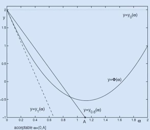
One way of defining this sufficient amount is by using the Armijo condition. Let $\Phi_k (\alpha) := f(x_k + \alpha s_k)$. The Armijo condition requires that $$ \Phi_k(\alpha_k) \leqslant y_\beta(\alpha_k) := \Phi_k(0) + \beta\alpha_k\Phi’(0), $$ for some $\beta \in (0, 1)$.
An algorithm that uses the Armijo condition will start with some large, initial step size $\alpha_k$, and backtracks (binary search style!) to find an $\alpha_k$ that satisfies the above condition. (What should the initial step size be? Sometimes we just start with 1 agnostically, but there are some very interesting methods for “guessing” a good starting value!)
Intuitively, what is the Armijo condition doing? Like the exact line-search, we are restricting $f$ to a line defined by the direction of $s_k$. This restricted version is $\Phi_k$. Exact line-search minimizes $\Phi_k$. However, here we are finding the line that is tangent to $\Phi_k$ at $0$, rotate it upwards by a small amount determined by $\beta$, and just find any point that is below this rotated line. The more we rotate the tangent, the easier it will be to find a point that lies below it, but also the more inaccurate (and suboptimal) the resulting step size may be.
The figure below may be helpful to better understand this. Notice that $\Phi(\alpha)$ is the restricted version of $f$, $y_1(\alpha)$ is the tangent to it at zero, and $y_{0.6}(\alpha)$ is its the rotated version. Selecting any point at which $\Phi$ is below this line will result in a “sufficiently good” step size.
Steepest Descent
Choosing $s_k$ to be the negative gradient and using any line-search method will give an algorithm that is often called the method of steepest descent. Notice that the line-search, be it exact or with Armijo-like conditions, is key here, as it allows us to show some nice convergence properties. The next theorem, showcases this.
Theorem: Let $f$ be sufficiently smooth (i.e., $\nabla f$ is Lipschitz continuous) and bounded from below. The method of steepest descent globally converges, meaning that $$ ||\nabla f(x_k)|| \to 0 \;\; \mathrm{as} \;\; k \to \infty. $$ Although steepest descent (SD) converges, it does so slowly. This is because SD is scale-dependent. Look at the Contour plots below and the evolution of the SD solution. In the first plot, SD (exact line-search) is able to find the minimizer in one step. However, if the problem becomes slightly ill-conditioned, as is in the second plot, it will take much longer for SD to converge.

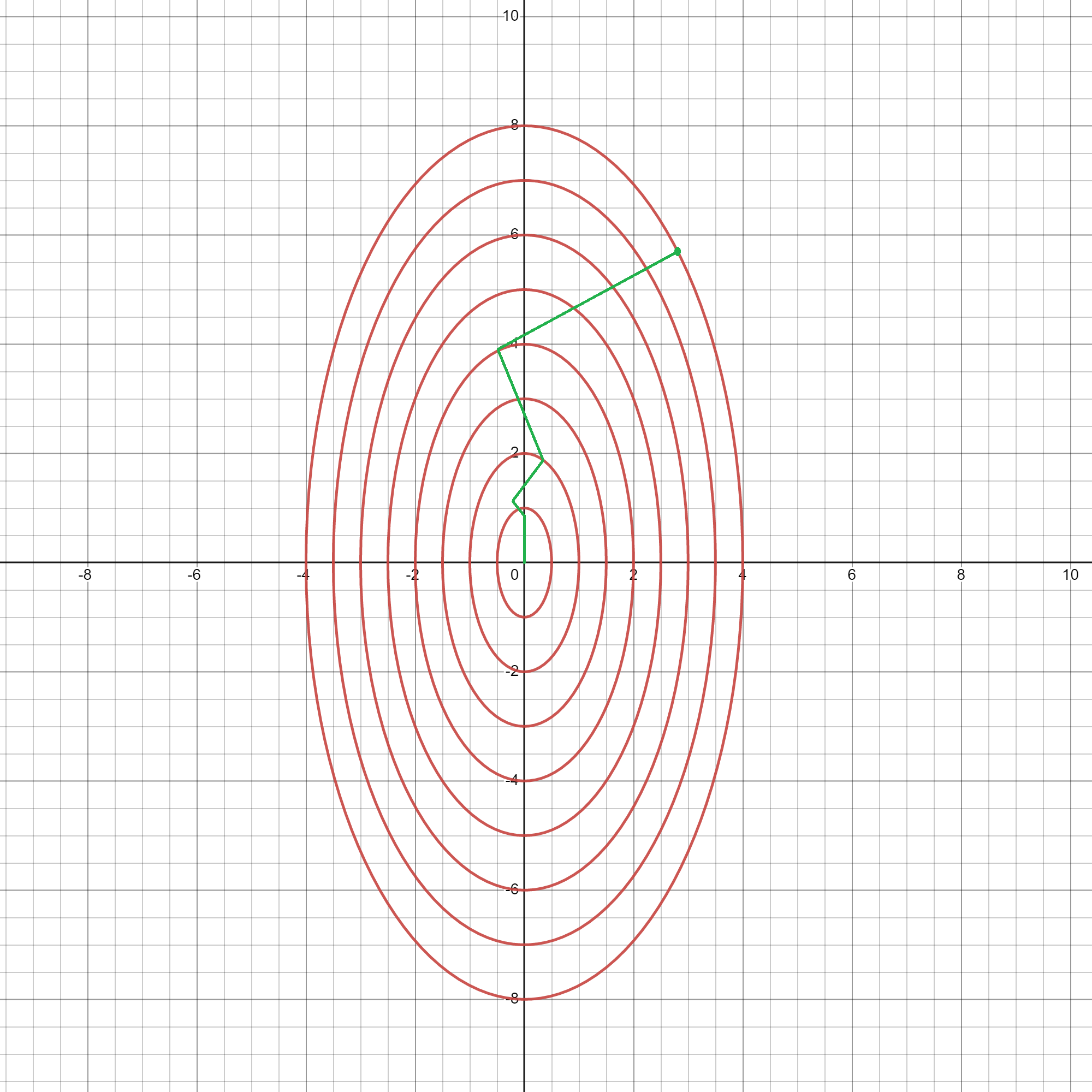
An Aside: SD converges linearly and the condition number of the Hessian matrix determines the rate of convergence for SD. This highlights the issue with SD: because it doesn’t take the curvature (Hessian) into account, it may perform poorly. As can be seen in the plots above, taking the direction of steepest descent is not always the best choice.
Beyond Steepest Descent
As we saw, SD with line-search can have very slow convergence rates. The simplest way for dealing with the ill-conditioning that was mentioned is to simply scale our variables (batch normalization in neural nets claims to be doing this!). Second order methods, headlined by the famous Newton’s method, use the Hessian (or an approximation of it) to automatically address this issue. In this section, general ideas behind these methods are presented without going into much details about the specificities of the algorithms.
Newton’s Method
Let’s revisit how we ended up with $-\nabla f(x_k)$ as the descent direction. In essence, we approximated $f$ near $x_k$ with a linear model. Using the Taylor expansion, this linear model was $$ m_k(s) = f(x_k) + \nabla f(x_k)^T s. $$ Now, if we want to minimize this function (subject to $||s|| = ||\nabla f(x_k)||$ to bound the values from below), we should let $s=-\nabla f(x_k)$. Therefore, the negative gradient direction was selected as the direction that minimizes the local linear model that we chose for $f$.
The idea behind Newton’s method is to use a second order approximation to $f$. Suppose $B_k$ is a symmetric positive-definite matrix and that we choose to locally approximate $f$ by $$ m_k(s) = f(x_k) + \nabla f(x_k)^T s +\frac{1}{2}s^TB_ks. $$ Because $B_k$ is positive-definite, this quadratic function has a unique minimum that can be found by: $$ \nabla_s m_k(s^*) = 0 \implies -\nabla f(x_k) = B_ks^*. $$ So, to find the direction of descent we must solve this system of linear equations for $s^*$.
One question remains, how should we choose $B_k$? First, notice that we need $B_k$ to be positive-definite to guarantee that $s^*$ is a descent direction: $$ s^T\nabla f(x_k) < 0 \implies -s^TB_ks < 0 \implies s^TB_ks >0. $$ If $\nabla^2 f(x_k)$ is positive-definite, we can let $B_k = \nabla^2 f(x_k)$ as this would result in the best quadratic approximation of $f$ (Taylor expansion). This choice gives raise to an algorithm known as the damped Newton method.
However, the Hessian need not be positive-definite, it may be that its positive-semidefinite. So this choice of $B_k$ requires $f$ to be locally strictly convex everywhere! Even if this is the case, we still need a number of additional assumptions to prove global convergence. To summarize, Newton’s method
- is scale-invariant (solves the issue with steepest descent),
- can speed up convergence (quadratic convergence) for functions with positive-definite Hessians,
- has no global convergence guarantees, even worse, it may not converge at all for some simple examples.
Modified Newton Method
When the Hessian is not positive-definite, we can “perturb” it a little so that it becomes sufficiently positive definite. In modified Newton method the descent direction is found by solving a slightly different system of linear equaitons: $$ (\nabla^2 f(x_k) + M_k)s_k = -\nabla f(x_k), $$ where $M_k$ is chosen such that $\nabla^2 f(x_k) + M_k$ is “sufficiently” positive-definite. Here, we will not get into the details of computing $M_k$.
This allows Newton’s method to be used with general objectives that don’t necessarily have positive-definite Hessians. However, we still need some additional assumptions to guarantee their global convergence.
Quasi-Newton Methods
When we don’t have access to second order derivatives, we can use a class of methods called quasi-Newton methods, to compute an approximation of the Hessian, $B_k \approx \nabla^2 f(x_k)$. A very general description of these methods is as follows: we start by an initial guess, $B_0$. After computing $s_k$ by solving $B_ks_k = -\nabla f(x_k)$ and setting $x_{k+1} = x_k + \alpha_ks_k$, we compute a (cheap) update $B_{k+1}$ of $B_k$.
Again, we don’t go into the details of how $B_k$ is updated. There are several methods that use this idea. BFGS and DFP are two of the most important ones that are considered to be state-of-the-art for unconstrained optimization.
Quasi-Newton methods are faster than Newton’s method, they require $\mathcal{O}(n^2)$ calculations per iteration as opposed to the $\mathcal{O}(n^3)$ required by Newton’s method. They also converge faster (in fewer iterations) compared to steepest descent methods, as they leverage curvature information.
Line-search Wrap-up
In this final section, let’s put all the things that we saw about line-search together so that we can have a clear idea of what line-search methods are doing.
At the $k$-th step, line-search methods locally approximate the non-convex objective function $f$ with a simple model $m_k$. This model can be linear, in which case it has the form $m_k(s) = f(x_k) + \nabla f(x_k)^Ts$ or quadratic, in which case it has the form $m_k(s) = f(x_k) + \nabla f(x_k)^Ts + \frac{1}{2}s^TB_k s$. When we have access to the Hessian, we can use $B_k = \nabla^2 f(x_k)$, otherwise, we can use estimates of the Hessian.
Once we have this model $m_k$, we use it to find a descent direction, $s_k$. This direction is found by minimizing the model, $m_k$. In the case of a linear model, this direction is $-\nabla f(x_k)$ and in the case of the quadratic model it is the solution to $B_ks_k = -\nabla f(x_k)$. Notice two important points:
- When we use a linear model, $m_k$ is not bounded from below. Therefore, we can’t minimize it. To address this issue, we actually solve the constrained optimization $\min_{s}m_k(s)$ subject to $||s||<\nabla f(x_k)$.
- When we use a quadratic model, $m_k$ is not bounded from below unless it is a convex, which is the case if and only if $B_k$ is positive-definite. So, when $B_k$ is not positive-definite, we perturb it. In essence, we locally approximate $f$ with a convex quadratic, even if $f$ is not locally convex. This means that our model may no longer be the most accurate local approximation.
Finally, when we have a descent direction we need to find a suitable step size $\alpha_k$ so that taking a step of this size in the descent direction results in a “sufficient decrease” in the value of $f$. To find this step size we use either exact line search or Armijo-like conditions.
This wraps-up our discussion of line-search methods.
Trust-region Methods
The basic idea behind line-search methods is “I know which direction I want to go, find me the largest step I can take in that direction to ensure sufficient progress in minimizing $f$”. Trust-region methods take the opposite approach; their methodology is “I know the maximum step size I want to take, find me the best direction to follow”. This nicely illustrates the main idea behind trust-region methods as well as its differences compared to line-search methods.
Let’s begin our discussion of trust-region methods (TR). Similar to line-search, we begin by approximating $f(x_k + s)$ by a quadratic model $$ m_k(s) = f(x_k) + \nabla f(x_k)^T s + \frac{1}{2} s^T B_k s, $$ where $B_k$ is some symmetric (but not necessarily positive-definite) approximation of $\nabla^2 f(x_k)$. This model has two possible issues:
- It may not resemble $f(x_k +s)$ for large values of $s$,
- It may be unbounded from below: if $m_k$ is not convex, it will be unbounded and we can’t meaningfully talk about minimize it.
Trust-region methods prevent bad approximations by “trusting” the model only in a trust region, defined by the trust-region constraint
$$
||s|| \leqslant \Delta_k
$$
for some appropriate radius $\Delta_k$.
This constraint also addresses the second issue by not allowing the model to be unbounded.
The Trust-region Subproblem: We refer to the minimization of the model subject to the trust region constraint as the trust-region subproblem: $$ \min_{s\in \R^n} m_k(s) \;\;\mathrm{subject\;to} \;\; ||s|| \leqslant \Delta_k $$ Notice that here, unlike in line-search, the model may be non-convex.
Solving The Trust-region Subproblem:
There are various efficient ways for computing (or approximating) the solution of this constrained optimization problem. Here, we just briefly mention a few popular strategies:
- We can solve this problem exactly, and find the global minimizer. This would result in a Newton-like trust-region method.
- In large-scale problems, we can solve it approximately, using iterative methods such as conjugate-gradient or Lancsoz method.
Now, let’s assume that we have the solution $s_k$ to the trust-region subproblem. How should we use it to take an optimization step?
The predicted model decrease from taking the step $s_k$ is $$ m_k(0) - m_k(s_k) = f(x_k) - m_k(s_k). $$ The actual function decrease is $$ f(x_k) - f(x_k + s_k). $$ Consider the ratio of these two $$ \rho_k := \frac{f(x_k) - f(x_k + s_k)}{f(x_k) - m_k(s_k)}. $$ If in the current trust-region $m_k$ is a good model for $f$, we expect $\rho_k$ to be close to $1$. If $\rho_k$ is much smaller than $1$, it means that our trust region is too large and the model can not accurately approximate $f$ in this region. This means that we have to decrease the radius of the trust region. So, the trust region radius $\Delta_k$ will be updated based on $\rho_k$:
- If $\rho_k$ is not too smaller than $1$, take an optimization step $x_{k+1} = x_{k} + s_k$ and increase the trust region radius, $\Delta_{k+1} \geqslant \Delta_k$.
- If $\rho_k$ is much smaller than $1$, shrink the trust region without taking any steps: $x_{k+1} = x_{k}$, $\Delta_{k+1} < \Delta_k$.
(One simple way to shrink or expand $\Delta_k$ is by multiplying or dividing by $2$)
What about convergence? Under similar assumptions to those of the steepest descent, this general recipe for trust-region optimization converges globally! But note that unlike steepest descent, we can use a wide variety of methods for computing the descent direction: we can use Newton or Quasi-Newton methods, approximate methods, etc.
This section ends by mentioning some remarks about line-search and trust-region methods.
- Quasi-Newton methods and approximate derivatives can be used within the trust-region framework (Note that we don’t need positive-definite updates for the Hessian)
- There are state-of-the-art implementations of both line-search and trust-region methods. Generally, they have similar performances and choosing between the two is now mostly a matter of taste.
Constrained Optimization
Preliminaries
In this chapter we move on to study constrained optimization problems. Again, we have an objective function $f: \R^n \to \R$ that we want to minimize. But now, we have a set of equality and inequality constraints that our solution must satisfy. These constraints are smooth, but can be very complicated functions. Furthermore, although each of them is smooth, their union may specify a feasible region with a lot of “rough edges”. Consider linear programming for instance: there all of the constraints are linear, but the feasible region can be a polygon with many sides and sharp corners. In fact, this is precisely what makes linear programming hard.
Mathematically, a constrained optimization problem is formulated as $$ \min_{x\in \R^n} f(x) \;\; \mathrm{subject\; to} \\ c_E(x) = 0, \\ c_I(x) \geqslant 0, $$ where $f: \R^n \to \R$ is a smooth objective function and $E, I$ are index sets. By $c_I(x) \geqslant 0$ we mean $c_i(x) \geqslant 0$ for all $i\in I$, and similarly for $c_E$. All of the constraints $c_i$ are smooth functions.
We refer to the set of points that satisfy the constraints as the feasible region, denoted by $\Omega$: $$ \Omega = {x\in \R^n: c_E(x) = 0, \; c_I(x) \geqslant 0} $$
Characterizing Solutions
As we saw in the first chapter, solutions to an unconstrained optimization problem could be characterized in terms of derivatives. In particular, we saw that any minimizer has to be an stationary point for $f$. This is not necessarily the case in constrained optimization. A minimizer may be a boundary point (located on the boundary of the feasible regions) in which case it doesn’t have to be an stationary point of $f$. The plot below shows an example of this where the global minimizer of the blue function within the region defined by the red lines is a boundary point with non-zero derivative.
The analogue of stationarity in constrained problems is the Karush-Kuhn-Tucker (KKT) conditions. KKT condition helps us characterize solutions in terms of derivatives. $$ \mathrm{unconstrained \; problems} \longrightarrow \hat{x}\;\mathrm{is \; stationary \; point}\; (\nabla f(\hat{x}) = 0) \\ \mathrm{constrained \; problems} \longrightarrow \hat{x}\;\mathrm{is \; KKT \; point} $$ To introduce the KKT conditions, we first need to define the Lagrangian function of a constrained optimization problem.
The Lagrangian function of a constrained optimization problem is defined as $$ \mathcal{L}(x, y, \lambda) := f(x) - \sum_{j\in E} {y_j c_j (x)} - \sum_{i\in I} {\lambda_i c_i(x)}. $$ The values $y, \lambda$ are known as Lagrange multipliers. The Lagrangian compresses the objective and the constraints of a problem into a single expression.
A point $\hat x$ is a KKT point of a constrained problem if multipliers $(\hat y, \hat \lambda)$ exist such that
- $\hat x$ is an stationary point of the Lagrangian for these multipliers, i.e., $\nabla_x \mathcal{L}(\hat x, \hat y, \hat \lambda) = 0$,
- the multipliers for inequalities are non-negative, i.e., $\hat \lambda \geqslant 0$,
- only active constraints matter at $\hat x$, i.e., for all $i\in I$, $\hat \lambda_i c_i (\hat x) = 0$,
- $\hat x$ is feasible, i.e., $c_E(\hat x) = 0$, $c_I(\hat x) \geqslant 0$.
Condition 3 may be a bit strange, so let’s focus on that a little. It asserts that $\hat\lambda_i c_i(\hat x)$ must be zero for all inequality constraints. This means that either $c_i(\hat x) = 0$ or otherwise, $\hat\lambda_i = 0$. If $c_i(\hat x) = 0$, it means that $\hat x$ is on the boundary of the region defined by the $i$-th inequality constraint. When this is the case, we call the $i$-th constraint “active”. Therefore, the multipliers must be zero for any inactive condition. This makes sense, because if a condition is inactive, it means that $\hat x$ is in the interior of the region determined by that condition (either on the feasible side or on the infeasible side). If this is the case, we are not concerned with that condition, because it is “far away” from us.
To further illustrate this, look at the example plotted in the beginning of this section. There we have two inequality constraints: $x- 2\geqslant 0$, $9-x \geqslant 0$. When we want to investigate the optimality of $\hat x = 2$ the first condition is active, as we are on the boundary of the region defined by this constraint. The second condition, in contrast, is inactive, as we are away from it’s boundary. To investigate the optimality of $\hat x$, it doesn’t matter if the second condition is $9-x\geqslant0$ or $1000 - x \geqslant 0$. So effectively, we don’t have to consider this condition. Therefore, the third condition requires the multiplier corresponding to this constraint to be zero, i.e., this condition is not included in the Lagrangian.
Also, note that the condition 4 ensures that we are on the “correct side” of inactive conditions.
With these explanations in mind, let’s take a closer look at condition 1. The gradient of the Lagrangian with respect to $x$ is $$ \nabla_x \mathcal{L}(\hat x, \hat y, \hat \lambda) = \nabla f(x) - \sum_{j\in E} {y_j \nabla c_j (x)} - \sum_{i\in I} {\lambda_i \nabla c_i(x)}. $$ If we take it to be zero, we get $$ \nabla_x \mathcal{L}(\hat x, \hat y, \hat \lambda) = 0 \\ \implies \nabla f(x) = \sum_{j\in E} {y_j \nabla c_j (x)} + \sum_{i\in I} {\lambda_i \nabla c_i(x)}. $$ In words, condition 1 is maintaining that at a KKT point, the gradient of the objective must be a linear combination of the gradients of (active) constraints.
A Caveat: In general, not every KKT point is an optimal point for the constrained optimization problem. We also need the constraints to satisfy some regularity assumptions known as constraint qualifications in order to derive necessary optimality conditions (for instance, the feasible region defined by the constraints must have an interior). A good news is that if the constraints are linear (as is the case for linear and quadratic programming), no constraint qualification is required.
Theorem [First order necessary conditions]: Under suitable constraint qualification, any local minimizer of a constrained optimization problem, is a KKT point.
Methods
Quadratic Penalty (Equality Constraints)
Let’s focus our attention on optimization problems that only have equality constraints. We can formulate these problems as $$ \min_{x\in\R^n} f(x) \;\;\mathrm{subject\;to} \;\; c(x) = 0, $$ where $f:\R^n\to\R$ and $c:\R^n\to\R^m$ are smooth functions.
One idea for solving such problems is to form a single, parametrized and unconstrained objective, whose minimizers approach the solutions to the initial problem as the parameter value varies.
The quadratic penalty function is one such function. It is defined as $$ \Phi_\sigma (x) := f(x) + \frac{1}{2\sigma}||c(x)||^2, $$ where $\sigma > 0$ is the penalty parameter. Now instead of solving the original problem, we solve the unconstrained minimization of $\Phi_\sigma$.
Notice that a minimizer of $\Phi_\sigma$ does not necessarily satisfy the constraint. But, as we let $\sigma \to 0$, we penalize infeasible points more and more, and force the solution to satisfy the constraint.
We could use any method for solving the unconstrained optimization of $\Phi_\sigma$ (line-search, trust-region, etc.).
Some consideration:
-
We typically use simple schedules like $\sigma_{k+1} = 0.1\sigma_k$ or $\sigma_{k+1} = \sigma_k^2$ to decrease $\sigma$.
-
Say we optimized $\Phi_{\sigma_k}$ and found a minimizer $x_k$. When we decrease the value of $\sigma_k$ and want to minimize $\Phi_{\sigma_{k+1}}$, we start the optimization from $x_k$. This kind of “warm starting” helps a lot in practice.
-
As $\sigma$ approaches zero, $\Phi_\sigma$ becomes very steep in the direction of the constraint’s gradients (See the figure below). As a result, the optimization of $\Phi_\sigma$ becomes ill-conditioned. This is something that we have to keep in mind when minimizing $\Phi_\sigma$. For instance, first order methods will probably not work well. Additionally, when we want to use trust-region methods, it’s best if we scale the trust region to account for the ill-conditioning of the problem.

-
Other effective ways of combating the ill-conditioning is to use change of variables or primal-dual variants, where we compute explicit changes in both $x$ and constraint multipliers $\lambda$.
Putting these ideas together, the quadratic penalty method has the following structure.
Quadratic Penalty Method(QP):
    Start with an initial value of 𝜎₀ > 0
    𝑘 = 0
    while not converged:
    	Choose 0 < 𝜎ₖ₊₁ < 𝜎ₖ
    	Starting from 𝑥ₖ⁽⁰⁾ (Possibly 𝑥ₖ⁽⁰⁾ = 𝑥ₖ), use an unconstrained minimization algorithm to find an approximate minimizer 𝑥ₖ₊₁ of Φ_𝜎ₖ₊₁
        𝑘 = 𝑘 + 1
Interior Point (Inequality Constraints)
Now let’s see how we can deal with inequality constraints. For the sake of simplicity, assume that we only have inequality constraints. So our problem can be written as $$ \min_{x\in\R^n} f(x) \;\;\mathrm{subject\;to} \;\; c(x) \geqslant 0, $$ where $f:\R^n\to\R$ and $c:\R^n\to\R^m$ are smooth functions.
Again, the idea is to turn this into an unconstrained optimization. **Barrier function** methods are one way of doing this. For $\mu > 0$, the corresponding **logarithmic barrier subproblem** is defined as $$ \min_{x\in \R^n} f_\mu := f(x) - \mu\sum_{i} \log c_i(x) \\ \mathrm{subject\; to} \;\; c(x) > 0. $$ Notice that in essence, this is an unconstrained optimization because the log barrier prevents the optimization algorithm to “go over” the constraint boundary. Let’s focus on this a bit more. How does the log transformation help us stay inside the feasible region? Consider what happens at the boundaries of the constraints. If we get close to the boundaries of the $i$-th constraint, the $\log$ term approaches $-\infty$. Thus, the value of the barrier function gets very large. This means that if we are at a point $x$ inside the feasible region and take an optimizing, step we will stay inside the feasible region because the barrier function increases sharply as we get closer to the boundary, provided that the optimizing step is not so large that we go over the barrier entirely (which can be guaranteed by forcing our line-search or trust-region method to respect $c(x) > 0$ when computing their step sizes). Therefore, we are guaranteed to stay inside the feasible region.
But there is a drawback to this. First, note that the $\log$ terms also change the landscape inside the feasible region. So a solution to the logarithmic barrier subproblem is not necessarily a local minimizer of the original objective. Furthermore, the local minimizer of the original objective may be on the boundary! If this is the case, the logarithmic subproblem will never reach it.
To solve these issues, we do something similar to what we did with the quadratic penalty function: We iteratively decrease $\mu$ and minimize $f_\mu$, warm-starting from the solution of the previous iteration.
The basic barrier method is presented below.
Basic Barrier Method(B):
    Start with an initial value of $\mu_0>0$
    𝑘 = 0
    while not converged:
    	Choose 0 < μₖ₊₁ < μₖ
    	Starting from a point 𝑥ₖ⁽⁰⁾ satisfying 𝑐(𝑥ₖ⁽⁰⁾) > 0 (Possibly 𝑥ₖ⁽⁰⁾ = 𝑥ₖ), use an unconstrained optimization algorithm to find an approximate minimizer 𝑥ₖ₊₁ of 𝑓_μₖ₊₁. Ensure that the optimizer doesn't take large steps that will result in an infeasible point.

        𝑘 = 𝑘 + 1
Some considerations:
- Interior point methods require us to find at least one feasible point to get started. This may not always be trivial!
- Because the barrier function blows up near the boundaries, optimizing $f_\mu$ is again ill-conditioned. The problem here is much worse than in penalty methods (the barrier function literally goes to infinity!), so much that we have to use primal-dual methods.
- In implementations, it is essential to keep iterates away from the boundaries early in the iterations. Otherwise, we may get trapped near the boundary which makes convergence very slow.
Derivative-Free Optimization
Consider the (unconstrained) optimization problem of minimizing $f:\R^n \to \R$. Even when $f$ is smooth, we may want to use derivative-free methods to solve this problem. This may be because:
- Exact first derivatives are unavailable: $f(x)$ may be given by a black box, propriety code or a simulation.
- Computing $f(x)$ for any given $x$ is expensive: $f(x)$ may be given by a time-consuming numerical simulation or lab experiments.
- Numerical approximation of $\nabla f(x)$ is expensive or slow: Using finite-differencing for estimating the gradient may be too expensive.
- The values of $f(x)$ are noisy: When evaluation of $f(x)$ is inaccurate. For example when $f(x)$ depends on discretization, sampling, inaccurate data, etc. Then the gradient information is meaningless.
What are some actual examples of such situations? One common and important case is hyperparameter tuning (e.g., in machine learning). In hyperparameter tuning derivative calculation is often impossible and evaluations are costly. Some other examples are parameter estimation, automatic error analysis, engineering design, molecular geometry, etc.
There are many derivative-free algorithms for optimization. Some examples are model-based methods, direct-search algorithms, pattern-search, Nelder-Mead and random search. These algorithms share some common characteristics:
- They only use objective function values to construct iterates.
- Do not compute an approximate gradient.
- Instead, they form a sample of points (less tightly clustered than in finite-differences) and use the associated function values to construct $x_{k+1}$. They also control the geometry of the sample sets.
- They try to approximate local solution with “few” function evaluations.
- Asymptotic speed is irrelevant as they don’t have any optimality condition for termination.
- They are suitable for non-smooth and global optimization.
There are also some limitations to these methods:
- They work best when the problem is small in scale (order of $10^2$ variables).
- The objective function $f$ must be quite smooth.
Model-Based Trust-Region Derivative-Free Optimization
To illustrate how derivative-free methods work, we briefly discuss a model-based method. They underlaying idea is similar to what we did in derivative-based unconstrained optimization. Essentially, we want to create models of $f$ that are not based on the gradient. This means that we can’t use Taylor models. So how are we to create such models? The idea is to create a model by interpolating $f$ on a set of appropriately chosen sample points.
Assume we have a sample set $Y = {y_1, \cdots, y_q}$ and that we have evaluated $f$ at these points. Furthermore, assume that $x_k \in Y$ is the current iterate which is the most optimal point in $Y$, i.e., $f(x_k)\leqslant f(y)$ for all $y\in Y$.
Our model $m_k(s)$ is again a simple linear or quadratic function of the following form $$ m_k(s) = c + s^Tg \;\;(+\frac{1}{2}s^THs), $$ where $c\in\R$, $g\in \R^n$ (, $H \in \R^{n\times n}$) are unknowns. To find these unknowns, we don’t use gradients or Hessians! Instead, we compute them to satisfy the interpolation conditions for the set of sampled points: $$ \forall y \in Y \;\; m_k(y - x_k) = f(y). $$ We need $q=n+1$ sample points to find the parameters of a linear model (i.e., $H=0$) and $q = \frac{(n+1)(n+2)}{2}$ points for a quadratic model.
Once we have a model, we use it just like in the derivative-based trust-region method, i.e., (because $m_k$ is non-convex) we add a trust-region constraint and solve $$ s_k = \arg \min_{s\in \R^n} m_k(s) \;\; \mathrm{subject \; to} \;\; ||s|| \leqslant \Delta_k. $$ We use $\rho_k$ to measure progress and proceed exactly like in the derivative-based method.
Because recomputing $m_k$ requires many new function evaluations, we instead update it by removing one point from the sample set, $Y$, and replacing it with a new point.
This is a rough sketch for a model-based, trust-region, derivative-free algorithm. But note that a complete algorithm is much more involved, we must
- make sure that the system of linear equations used for finding model parameters is non-singular,
- monitor the geometry of $Y$ to help with conditioning,
- have suitable strategies for adding and removing points from $Y$,
- …
An Aside: One thing to note here is that we are not limited to linear and quadratic models. As long as we can minimize the model with the trust-region method, we are good to go! So based on the geometry of $f$, if we think that say, a sinusoidal function can better locally approximate it, we can use it as our model. Or if the number of variables, $n$, is too large, we may constrain $H$ to be a rank $1$ matrix or $g$ to be a sparse vector, thus reducing the number of parameters of the model.